


Spectral analysis of Direct Numerical Simulation data
with Matlab
Felix Dietzsch
a
a
Institut f¨ur Chemieingenieurwesen und Energieverfahrenstechnik,
Fuchsm¨uhlenweg 9, Reiche Zeche, 09599 Freiberg.
T +49 3731 394212, k Felix.Dietzsch@vtc.tu-freiberg.de
Contents
1 Contents 1
2 Clear complete workspace 1
3 Read data files 2
4 Set necessary parameters 3
5 Compute 3D spectrum 3
6 Compute dissipation and turbulent kinetic energy 8
7 Kolmogorov properties 10
8 Compute correlations 10
1. Contents
• Clear complete workspace
• Read data files
• Set necessary parameters
• Compute 3D spectrum
• Compute dissipation and turbulent kinetic energy
• Kolmogorov properties
• Compute correlations
2. Clear complete workspace
If you start a new Matlab project it is always a goot idea to clear the complete
workspace and command window. Since Matlab does not automatically open
1

new figure windows each time a plot is invoked we should close all remaining
figure windows. Also very important is to tell Matlab where to find the
functions we will use in our project. This is done by adding the functions
folder with path('./functions',path) to the Matlab search path.
display(’Clear workspace ...’)
path(’./functions’,path) % add directory the Matlab path
close all % close all figures
clear all % clear workspace
clc % clear command window
datadir=’data/stuttgart/’; % data directory
flag=’3D’;
%set(0,’DefaultFigureWindowStyle’,’docked’)
3. Read data files
During the evaluation of the function
ReadData
all velocity files necessary for
the calculation of the spectrum and the correlation coefficients are read. In
addition the import operations are enclosed in a
tic;. . . ;toc
block which
measures the time needed for reading the ASCII data. Although the ASCII
data format ist not the best choice in terms of speed and size, we will use it
since other methodologies require additional knowledge of data processing.
Just for your information a very famous and highly portable data format is
hdf5. It is a software library that is available for a range of computer platforms,
from laptops to massively parallel systems and implements a high-level API
(Application programming interface) with C, C
++
, Fortran 90, and Java
interfaces. Besides its hierarchical structure it is highly optimized for parallel
I/O operations and can be read by nearly all data processing/visualization
tools.
display(’Read data ...’)
[uvel,vvel,wvel,time_read,dim] = ReadData(datadir,flag,...
’uvel’,...
’vvel’,...
’wvel’);
2

1 function [uvel,vvel,wvel,time,dim] = ReadData(datadir,...
2 flag,...
3 u name,...
4 v name,...
5 w name)
6 tic; % enable timer
7 uvel=importdata([datadir,'/',u name]);
8 vvel=importdata([datadir,'/',v name]);
9 wvel=importdata([datadir,'/',w name]);
10 time = toc; % end timer
11 if strcmp(flag,'3D')
12 dim=round((size(uvel,1))ˆ(1/3));
13 end
14 end
4. Set necessary parameters
For further computations we have to to define some parmeters of the DNS
simulation.
display(’Set parameters ...’)
[u,v,w,Lx,nu]=Params(uvel,vvel,wvel,dim);
1 function [u,v,w,Lx,nu]=Params(uvel,vvel,wvel,dim)
2 Lx=2
*
pi; %edge length
3 nu=1.7e−5; % viscosity
4 u=reshape(uvel,dim,dim,dim); % reshape to 3D
5 v=reshape(vvel,dim,dim,dim);
6 w=reshape(wvel,dim,dim,dim);
7 clear uvel vvel wvel % save memory
8 end
5. Compute 3D spectrum
The core of the code is contained in the function
PowerSpec
. It computes the
three dimensional energy spectrum from the given velocity fields, obtained
from a direct numerical simulation. Although the theoretical analysis is
3

relatively demanding compared to one dimensional spectra its worth investing
the effort. The theory of one dimensional spectra relies on the assumption
that the propagation of spectral waves (
κ
1
) is in the direction of the observed
velocity fields or to say it differently one dimensional spectra and correlation
functions are Fourier transform pairs. The theory of correlation functions
will be discussed in section 8. A key drawback of this theory is that the
calculated spectrum has contributions from all wavenumbers
κ
, so that the
magnitude of
κ
can be appreciably larger than
κ
1
. This phenomenon is called
aliasing. In order to avoid these aliasing effects is also possible to produce
correlations that involve all possible directions. The three dimensional Fourier
transformation of such a correlation produces a spectrum that not only
depends on a single wavenumber but on the wavenumber vector
κ
i
. Though
the directional information contained in
κ
i
eliminates the aliasing problem the
complexity makes a physical reasoning impossible. For homogeneous isotropic
turbulence the situation can be considerably simplified. From the knowledge
that the velocity field is isotropic it can be shown that the velocity spectrum
tensor is fully determined by
Φ
ij
(κ) = A(κ)δ
ij
+ B(κ)κ
i
κ
j
, (1)
where
A
(
κ
) and
B
(
κ
) are arbitrary scalar functions. Since we assume in-
compressible fluids (mathematically expressed by
∇ · u
= 0 or
κ
i
u
i
= 0 the
following condition holds
κ
i
Φ
ij
(κ) = 0. (2)
It can be shown that this yields a relation between A and B by means of
B(|κ|) = −
A(|κ|)
(|κ|)
2
(3)
In the end this gives a relation between the three dimensional energy spectrum
function E(|κ|) and the velocity spectrum tensor Φ
ij
.
Φ
ij
=
E(|κ|)
4π (|κ|)
2
δ
ij
−
κ
i
κ
j
(|κ|)
2
(4)
The question is now how the remaining variable (
A
or
B
) can be determined.
Regarding the turbulent kinetic energy we know that
k =
∞
ˆ
−∞
E(|κ|) dk =
X
κ
E(κ) =
X
κ
1
2
hu
∗
(κ) u(κ)i =
∞
˚
−∞
1
2
Φ
ii
(κ) dκ. (5)
4
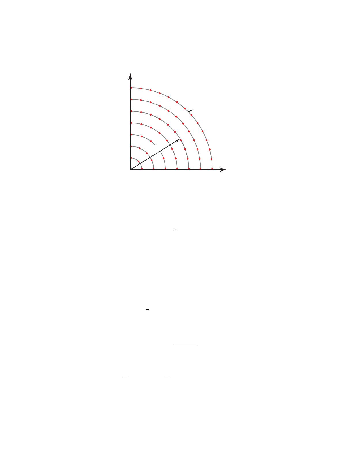
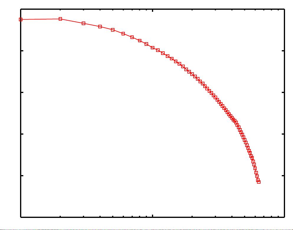
κ
1
|
𝛋|=k
E(|𝛋|)
κ
2
Fig. 1: Illustration of the two dimensional shell integration
Comparing the second and last expression we get
E(|κ|) =
‹
1
2
Φ
ii
(κ) dS(κ). (6)
This integral can be solved analytically by utilizing again the assumption
of isotropy. For these kind of flows the energy spectrum function can be
regarded as the sum of kinetic energy (in wave number space) on different
energy levels. Each of these energy levels is denoted by a spherical shell in
wave number space. Since the surface of a sphere is completely determined
by its radius the surface integral can be solved analytically. The idea of this
integration is illustrated in Fig. ??. As a result of this one gets
E(|κ|) =
‹
1
2
Φ
ii
(κ) dS(κ) = 4π(|κ|)
2
Φ
ii
(|κ|). (7)
Introducing this relation to equations
(1)
and
(3)
one arrives at an expression
for the variable B.
B = −
E(|κ|)
4π(|κ|)
2
(8)
Together with the approximation of the integral of Φ (equation (5))
∞
˚
−∞
1
2
Φ
ii
(κ) dκ ≈
1
2
X
κ
Φ
ii
(κ) ∆κ
x
∆κ
y
∆κ
z
, (9)
5


