没有合适的资源?快使用搜索试试~ 我知道了~
斯坦福机器学习讲义,学习机器学习的最佳入门课程,视频连接http://open.163.com/special/opencourse/machinelearning.html
资源推荐
资源详情
资源评论
CS229 Lecture notes
Andrew Ng
Supervised learning
Lets start by talking about a few examples of supervised learning problems.
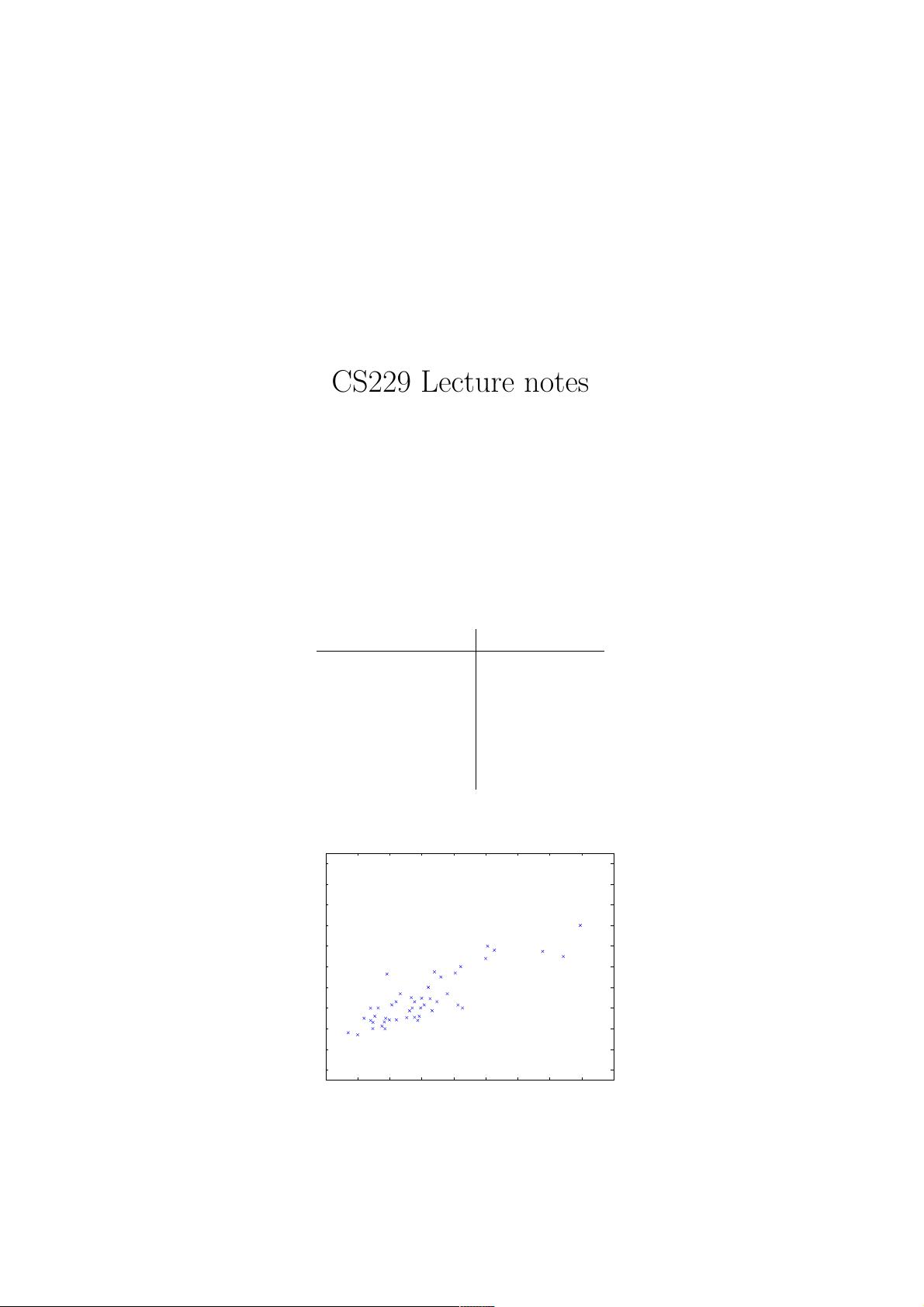
Suppose we have a dataset giving the living areas and prices of 47 houses
from Portland, Oregon:
Living area (feet
2
) Price (1000$s)
2104 400
1600
330
2400
369
1416
232
3000
540
.
.
.
.
.
.
We can plot this data:
500 1000 1500 2000 2500 3000 3500 4000 4500 5000
0
100
200
300
400
500
600
700
800
900
1000
housing prices
square feet
price (in $1000)
Given data like this, how can we learn to predict the prices of other houses
in Portland, as a function of the size of their living areas?
1
CS229 Winter 2003 2
To establish notation for future use, we’ll use x
(i)
to denote the “input”
variables (living area in this example), also called input features,andy
(i)
to denote the “output” or target variable that we are trying to predict
(price). A pair (x
(i)
,y
(i)
) is called a training example, and the dataset
that we’ll be using to learn—a list of m training examples {(x
(i)
,y
(i)
); i =
1,...,m}—is called a training set. Note that the superscript “(i)” in the
notation is simply an index into the training set, and has nothing to do with
exponentiation. We will also use X denote the space of input values, and Y
the space of output values. In this example, X = Y = R.
To describe the supervised learning problem slightly more formally, our
goal is, given a training set, to learn a function h : X !→ Y so that h(x)isa
“good” predictor for the corresponding value of y. For historical reasons, this
function h is called a hypothesis. Seen pictorially, the process is therefore
like this:
Training
set
house.)
(living area of
Learning
algorithm
h
predicted yx
(predicted price)
of house)
When the target variable that we’re trying to predict is continuous, such
as in our housing example, we call the learning problem a regression prob-
lem. When y can take on only a small number of discrete values (such as
if, given the living area, we wanted to predict if a dwelling is a house or an
apartment, say), we call it a classification problem.
3
Part I
Linear Regression
To make our housing example more interesting, lets consider a slightly richer
dataset in which we also know the number of bedrooms in each house:
Living area (feet
2
)
#bedrooms Price (1000$s)
2104 3 400
1600
3 330
2400
3 369
1416
2 232
3000
4 540
.
.
.
.
.
.
.
.
.
Here, the x’s are two-dimensional vectors in R
2
. For instance, x
(i)
1
is the
living area of the i-th house in the training set, and x
(i)
2
is its number of
bedrooms. (In general, when designing a learning problem, it will be up to
you to decide what features to choose, so if you are out in Portland gathering
housing data, you might also decide to include other features such as whether
each house has a fireplace, the number of bathrooms, and so on. We’ll say
more about feature selection later, but for now lets take the features as given.)
To perform supervised learning, we must decide how we’re going to rep-
resent functions/hypotheses h in a computer. As an initial choice, lets say
we decide to approximate y as a linear function of x:
h
θ
(x)=θ
0
+ θ
1
x
1
+ θ
2
x
2
Here, the θ
i
’s are the parameters (also called weights) parameterizing the
space of linear functions mapping from X to Y. When there is no risk of
confusion, we will drop the θ subscript in h
θ
(x), and write it more simply as
h(x). To simplify our notation, we also introduce the convention ofletting
x
0
=1(thisistheintercept term), so that
h(x)=
n
!
i=0
θ
i
x
i
= θ
T
x,
where on the right-hand side above we are viewing θ and x both as vectors,
and here n is the number of input variables (not counting x
0
).
Now, given a training set, how do we pick, or learn, the parameters θ?
One reasonable method seems to be to make h(x) close to y, at least for
4
the training examples we have. To formalize this, we will define a function
that measures, for each value of the θ’s, how close the h(x
(i)
)’s are to the
corresponding y
(i)
’s. We d efine the cost function:
J(θ)=
1
2
m
!
i=1
(h
θ
(x
(i)
) − y
(i)
)
2
.
If you’ve seen linear regression before, you may recognize this as the familiar
least-squares cost function that gives rise to the ordinary least squares
regression model. Whether or not you have seen it previously, lets keep
going, and we’ll eventually show this to be a special case of a much broader
family of algorithms.
1 LMS algorithm
We want to choose θ so as to minimize J(θ). To do so, lets use a search
algorithm that starts with some “initial guess” for θ, and that repeatedly
chan ges θ to make J(θ) smaller, until hopefully we converge to a value of
θ that minimizes J(θ). Specifically, lets consider the gradient descent
algorithm, which starts with some initial θ, and repeatedly performs the
update:
θ
j
:= θ
j
− α
∂
∂θ
j
J(θ).
(This update is simultaneously performed for all values of j =0,...,n.)
Here, α is called the learning rate. This is a very natural algorithm that
repeatedly takes a step in the direction of steepest decrease of J.
In order to implement this algorithm, we have to work out what is the
partial derivative term on the right hand side. Lets first work itoutforthe
case of if we have only one training example (x, y), so that we can neglect
the sum in the definition of J. We have:
∂
∂θ
j
J(θ)=
∂
∂θ
j
1
2
(h
θ
(x) − y)
2
=2·
1
2
(h
θ
(x) − y) ·
∂
∂θ
j
(h
θ
(x) − y)
=(h
θ
(x) − y) ·
∂
∂θ
j
"
n
!
i=0
θ
i
x
i
− y
#
=(h
θ
(x) − y) x
j
5
For a single training example, this gives the update rule:
1
θ
j
:= θ
j
+ α
$
y
(i)
− h
θ
(x
(i)
)
%
x
(i)
j
.
The rule is called the LMS update rule (LMS stands for “least mean squares”),
and is also known as the Widrow-Hoff learning rule. This rule has several
properties that seem natural and intuitive. For instance, the magnitude of
the update is proportional to the error term (y
(i)
− h
θ
(x
(i)
)); thus, for in-
stance, if we are encounter ing a training example on which our prediction
nearly matches the actual value of y
(i)
, then we find that there is little need
to change the parameters; in contrast, a larger ch ange to the parameters will
be made if our prediction h
θ
(x
(i)
) has a large error (i.e., if it is very far from
y
(i)
).
We’d derived the LMS rule for when t here was only a single training
example. There are two ways to modify this method for a training set of
more than one example. The first is replace it with the followingalgorithm:
Repeat until convergence {
θ
j
:= θ
j
+ α
&
m
i=1
$
y
(i)
− h
θ
(x
(i)
)
%
x
(i)
j
(for every j).
}
The reader can easily verify that the quantity in the summation in the update
rule above is just ∂J (θ)/∂θ
j
(for the original definition of J). So, this is
simply gradient descent on the original cost function J. This method looks
at every example in the entire training set on every step, and is called batch
gradient descent. Note that, while gradient descent can be susceptible
to local minima in general, the optimization problem we have posed here
for linear regression has only one global, and no other local, optima; thus
gradient descent always converges (assuming the learning rate α is not too
large) to the global minimum. Indeed, J is a convex quadratic function.
Here is an example of gradient descent as it is run to minimize a quadratic
function.
1
We use the notation “a := b” to denote an operation (in a computer program) in
which we set the value of a variable a to be equal to the value of b. In other words, this
operation overwrites a with the value of b. In contrast, we will write “a = b” when we are
asserting a statement of fact, that the value of a is equal to the value of b.
剩余133页未读,继续阅读
资源评论
qiuqiu374
- 粉丝: 1
- 资源: 1
上传资源 快速赚钱
- 我的内容管理 展开
- 我的资源 快来上传第一个资源
- 我的收益 登录查看自己的收益
- 我的积分 登录查看自己的积分
- 我的C币 登录后查看C币余额
- 我的收藏
- 我的下载
- 下载帮助
最新资源
- 通道处理过程的模拟通常涉及对通道处理机制的理解与实现.txt
- Flume进阶-自定义拦截器jar包
- Dubins曲线算法讲解和在运动规划中的使用.pdf
- 上市公司-股票性质数据-工具变量(民企、国企、央企)2003-2022年.dta
- 上市公司-股票性质数据-工具变量(民企、国企、央企)2003-2022年.xlsx
- Reeds+Shepp曲线算法讲解和实现.pdf
- 毕业设计基于SpringBoot+MyBatisPlus+MySQL+Vue的外卖配送信息系统源代码+数据库
- 词向量(Word Embeddings)是自然语言处理(NLP)领域的一种重要技术.txt
- Surfer,线性函数
- MyBatis 的动态 SQL 是其核心特性之一.txt
资源上传下载、课程学习等过程中有任何疑问或建议,欢迎提出宝贵意见哦~我们会及时处理!
点击此处反馈
安全验证
文档复制为VIP权益,开通VIP直接复制
信息提交成功