


1
Path Planning
FINAL PROJECT REPORT
For course:
Projects in Computer Science and Engineering
(June 10
th
, 2017)
HALMSTAD UNIVERSITY
Lu Han
SUPERVISOR
Jennifer David & Hassan Nemati

2
TABLE OF CONTENTS
TABLE OF CONTENTS ..................................................................................................................................................2
1.
INTRODUCTION ....................................................................................................................................................3
2.
METHOD ...............................................................................................................................................................3
2.1
STATIC SITUATION ...........................................................................................................................................4
2.1.1
PRM ............................................................................................................................................................4
2.1.2
DIJKSTRA ........................................................................................................................................................5
2.1.3
A STAR .........................................................................................................................................................7
2.1.4
COMPARE DIJKSTRA AND A STAR ...........................................................................................................8
2.2
DYNAMIC SITUATION ......................................................................................................................................9
2.2.1
D STAR ........................................................................................................................................................9
3.
EXPERIMENT AND RESULTS ..........................................................................................................................9
3.1
MAPS ...............................................................................................................................................................9
3.1.1
LOGICAL MAP ..............................................................................................................................................10
3.1.2
MAP FOR SMART HOME .........................................................................................................................10
3.2
STATIC SITUATION ........................................................................................................................................11
3.2.1
PRM .........................................................................................................................................................11
3.2.1.1
PRM IN LOGICAL MAP ...........................................................................................................................11
3.2.1.2
PRM IN SMART HOME MAP .................................................................................................................12
3.2.2
DIJKSTRA .....................................................................................................................................................13
3.2.2.1
DIJKSTRA IN LOGICAL MAP ...................................................................................................................13
3.2.2.2
DIJKSTRA IN SMART HOME MAP ..........................................................................................................14
3.2.3
ASTAR .......................................................................................................................................................14
3.2.3.1
A STAR IN LOGICAL MAP .......................................................................................................................14
3.2.3.2
ASTAR IN IMAGE MAP ............................................................................................................................15
3.3
DYNAMIC SITUATION ....................................................................................................................................16
3.3.1
D STAR ......................................................................................................................................................17
3.4
GUI DEVELOPMENT IN MATLAB: .....................................................................................................17
4.
CONCLUSION ......................................................................................................................................................19
REFERENCES ..............................................................................................................................................................20

3
1. INTRODUCTION
Path planning is an important primitive for autonomous mobile robots. The typical
path planning problem is to find a collision-free path from the start point to a specific
target point [1] in an environment with obstacles, according to certain evaluation
criteria (the shortest route, the least time, etc.)[2]. The robot should be able to move
safely, without collision through all the obstacles. The path planning problem can be
called collision avoidance planning problem as well [3].
The problem of path planning is finding a path in a static or dynamic environment,
for example, a maze, graph and road. Path planning lets the robots plan in the
environment with obstacles, then find the optimal path to avoid collision [4].
Researchers distinguish between various methods used to solve the path planning
problem according to two factors, the environment type (i.e., static or dynamic) [5]
the path planning algorithms (i.e., global or local) [6]
In this report, I will use simulation tools to analysis different path planning
algorithms under different environmental scenarios and do a comparative study with a
user interface developed in Matlab.
2. METHOD
Path planning can be divided into two types; one is global path planning in a static
environment and the other is local path planning in a dynamic environment.
In global path planning, the static environment is defined as an environment which
contains static objects only with the moving robot itself, while in local path planning,
the dynamic environment is defined as an environment that contains moving objects
like human beings, moving machines, or other moving robots. [7]
In global path planning, the robot needs to know all the environment information
and all terrain should be static, then according to the corresponding path planning
algorithm, the shortest path is found, while in local path planning, the robot needs to
collect real-time (online) environment information by sensors, then determine the
location of the robot in the map and the distribution of obstacles (localization), so that
the robot can find the optimal path from the current location to the goal point. In other
words, the algorithm is capable of producing a new path in response to environmental
changes [8] at every instant.
The path planning problem includes environment or map representation, path
searching (planning) and path smoothing in general.
1) Environment modelling or map representation.
The robot interprets the map of the environment in different ways. In this report, I
have two kinds of map, one is a logical map (which is hand drawn by myself) and the
other map is a .png image of the real environment.
2) Path searching or path planning
Path searching or path planning is finding the optimal path by different algorithms
based on the map representation.
3) Path smoothing
The path we find through corresponding method might not be a viable path that the
robot can pass through, it looks blocky and is not suited if you move your units with
floating point datatypes. So the path requires further processing and smoothing. In this
case, we can use inflated function to inflate the map with the robot radius first, after
4
getting the path, we choose some points in the path and generate more points between
two points, then the robot doesn’t need to cover all the point in the path and can avoid
sharp point location.
The robot's hand, arm, or body travels through the external world of the obstacle,
and when it reaches a certain target position, it is necessary to determine an optimized
travel path that does not collide in space. The measure of a good or bad planning
process mainly refers to two factors: collision free and efficiency.
Collision free: The main consideration is to avoid collision problems, also known
as collision-avoidance path planning.
Efficient: The main consideration is the path optimization problem. Try to make the
robot's hand, arm, or body in the possible shortest time reach the target location.
2.1 STATIC SITUATION
According to the feature of environmental information, path planning can be
divided into discrete domain path planning and continuous domain path planning. The
problem of path planning in discrete domain situation is roughly divided into global
planning and local planning. Due to the discrete domain path planning doesn’t care
much about the changing environment in local planning, so local path planning with
discrete domain can be regarded as global path planning in static situation.
PRM is a discrete domain path planning method, whereas Dijkstra and A star are
continuous domain path planning methods.
2.1.1 PRM
The probabilistic roadmap planner [9] is one of the mobile robot path planning
method which is based on random search to solve the problem of finding a path from
start location to a goal location without collision under static environment.
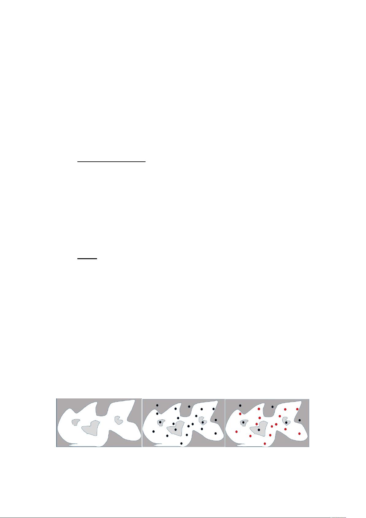
The basic idea of PRM is to generate specific number of random points in the map,
check if the linear segment between two points is within the distance of connection
and there is no obstacle in the line segment, and then connect these two points.
After
connecting all the segments in the map, we will get a connected network. The
iteration ends when the start and the end point are selected in the randomly
generated network. Then a simple search is run in this network from the start point to
the goal point to get an obstacle-free path without any collision. If the start point or
the goal point is not in the connect network, then the algorithm returns an empty array.
Also increasing the number of nodes and connection distances can raise the possibility
of finding path [10]. Hence, this method is probabilistically complete. This algorithm
is illustrated in Fig 2.1.1.1-2.1.1.4
(a)
(b)
(c)
Figure 2.1.1.1 Pick coordinates randomly and get available points.
5
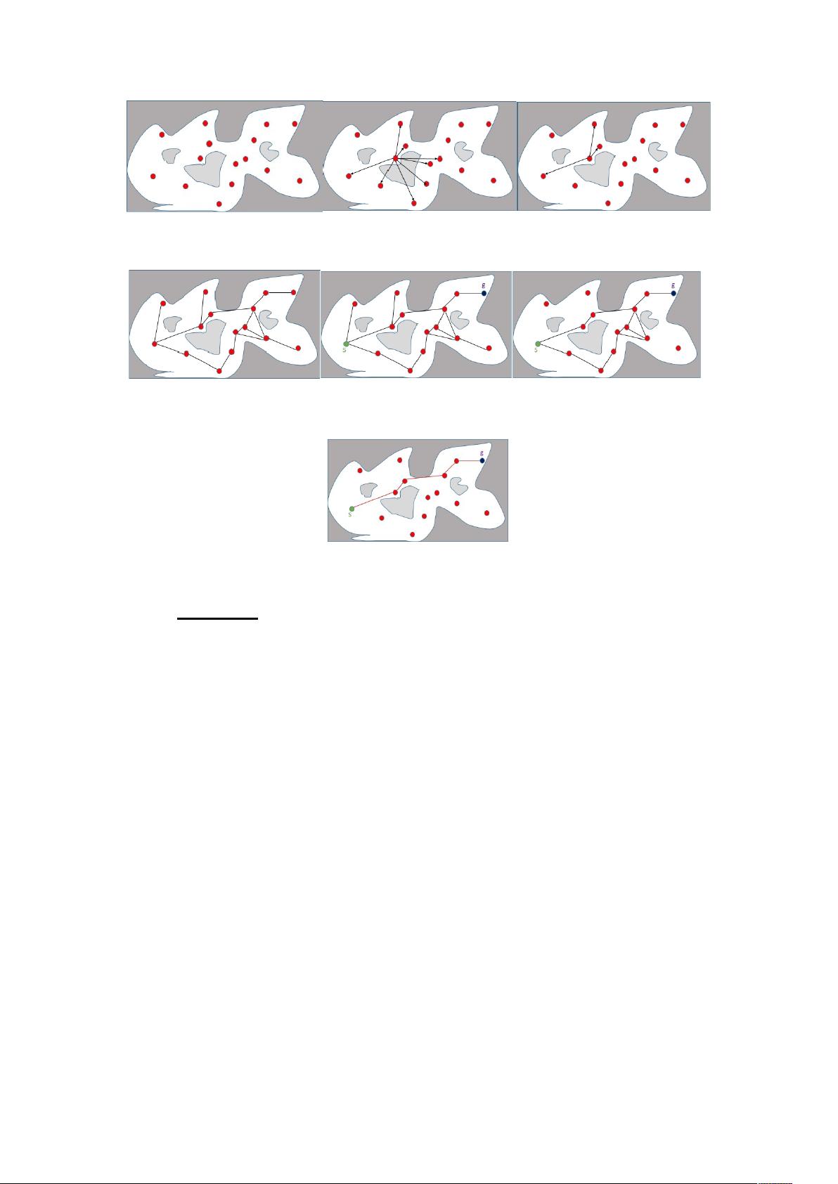
(a) (b) (c)
Figure 2.1.1.2 Connect collision-free neighbors.
(a)
(b)
(c)
Figure 2.1.1.3 Get all collision-free paths from start point to goal point.
Figure 2.1.1.4: Get the shortest path from start point to goal point.
2.1.2 DIJKSTRA
The Dijkstra algorithm is a typical shortest path algorithm which is used to
calculate the shortest path of a node to all other nodes. The main feature is in
expanding from the starting point to the next layer, until reach the goal point. Dijkstra
algorithm calculates the optimal shortest path always, but it traverses to all the nodes
around which makes the Dijkstra algorithm has a low efficiency [11].
The basic idea of Dijkstra algorithm is: Assuming G=(V,E) is a weighted directed
graph with E edges and the vertices as V. The vertex set V is further divided into two
groups, the first group has the list of all the shortest path in the vertex set, which is S,
the initial S has only one source point, and each time a shortest path is obtained, this
new vertex will be added to the set S until all the vertices are added to the S; the
second group is the set of vertices that do not determine the shortest path, which is U.
Then add all the vertices from U to S is sorted in the order of their shortest path
length. During this process, the shortest path length of the vertices from the source
point v to the S is always smaller than the shortest path length from any of the vertices
from the source point v to U. It should be noted that each vertex corresponds to a
distance, the distance from the vertex in S is the shortest path length from v to the
vertex, and the distance from the vertex in U is current path length from v to the
vertex. This is explained in figure 2.1.2.1
(1) Initially, S only contains the source point, S =[v], the distance of v is zero. U
contains the other vertices except v, the vertex u in U is the weight for the edge.
(2) Select a vertex k with the smallest distance from U, and add k to S, the selected
distance is the shortest path from v to k.


