


1 (2)
11.14
Department of Information Technology
Faculty of Mathematics and Natural Sciences
University of Turku
Department of Microelectronics
School of Information Science and Technology
Fudan University
Exercise 6: Parametrisable Parallel Multiplier
Background
Multiplication as an operation is used in very different applications. The actual implementation
in hardware depends on the constraints - available resources, calculation time, etc. The block
multipliers have rather simple and very regular internal structure. They are known also as
matrix multipliers because of the structure.
It can be said that very many structures of parallel multipliers base on a well-known
mathematical concept - multiplication of polynomials. An n-bit unsigned number can be always
represented as a polynomial:
(X
n-1
X
n-2
...X
2
X
1
X
0
)
2
= X
n-1
* 2
n-1
+ X
n-2
* 2
n-2
+ ... + X
2
* 2
2
+ X
1
* 2
1
+ X
0
* 2
0
(for example 1101 =1* 2
3
+ 1* 2
2
+ 0 * 2
1
+ 1 * 2
0
=8+4+0+1=13)
and the multiplication of two polynomials x and y becomes:
x*y = x
n-1
*y
m-1
*2
n+m-2
+ (x
n-1
* y
m-2
+ x
n-2
*y
m-1
)*2
n+m-3
+
… + (x
1
*y
0
+x
0
*y
1
)*2
1
+ (x
0
*y
0
) * 2
0
where a has n bits and b has m bits.
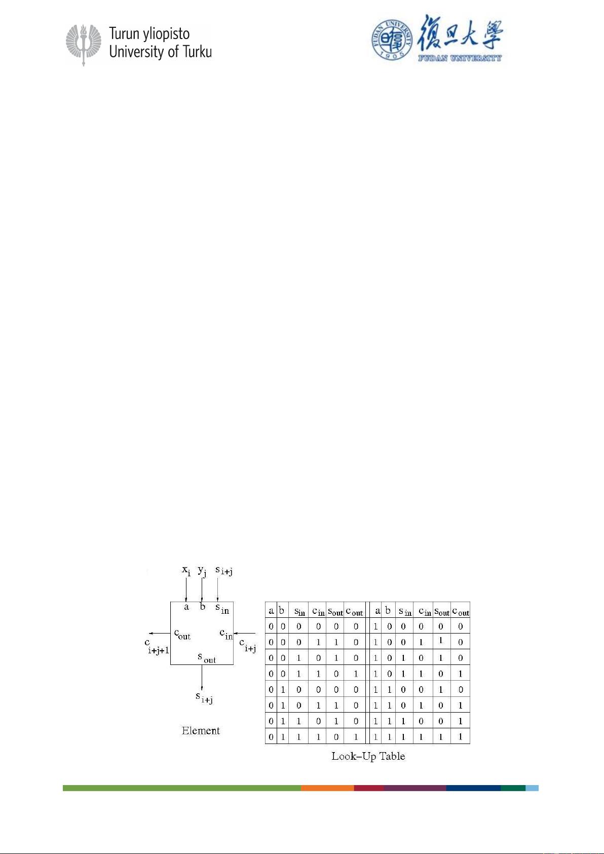
A typical element of such kind of multipliers is a 1-bit multiplier with additional inputs/outputs
to propagate sum and carry. Its inputs are x and y for data, sin for sum-in, cin for carry-in and
its outputs are sout for sum-out and cout for carry-out. You can use the following dataflow
model to calculate sout and cout
pp <= a AND b;
cout <= (pp AND sin) OR (pp AND cin) OR (sin AND cin);
sout <= pp XOR sin XOR cin;
Indexes on wires match the place in the matrix, i.e., bits with indexes i and j calculate sum with
weight 2
i+j
and carry for the next level (2
i+j+1
), and require partial sum and carry of the same
level (index i+j).


