没有合适的资源?快使用搜索试试~ 我知道了~
Numerical Computing with MATLAB: least squares
需积分: 0 5 下载量 186 浏览量
2009-08-08
10:35:50
上传
评论
收藏 216KB PDF 举报
温馨提示
试读
27页
Numerical Computing with MATLAB
资源详情
资源评论
资源推荐
Chapter 5
Least Squares
The term least squares describes a frequently used approach to solving overdeter-
mined or inexactly specified systems of equations in an approximate sense. Instead
of solving the equations exactly, we seek only to minimize the sum of the squares
of the residuals.
The least squares criterion has important statistical interpretations. If ap-
propriate probabilistic assumptions about underlying error distributions are made,
least squares produces what is known as the maximum-likelihood estimate of the pa-
rameters. Even if the probabilistic assumptions are not satisfied, years of experience
have shown that least squares produces useful results.
The computational techniques for linear least squares problems make use of
orthogonal matrix factorizations.
5.1 Models and Curve Fitting
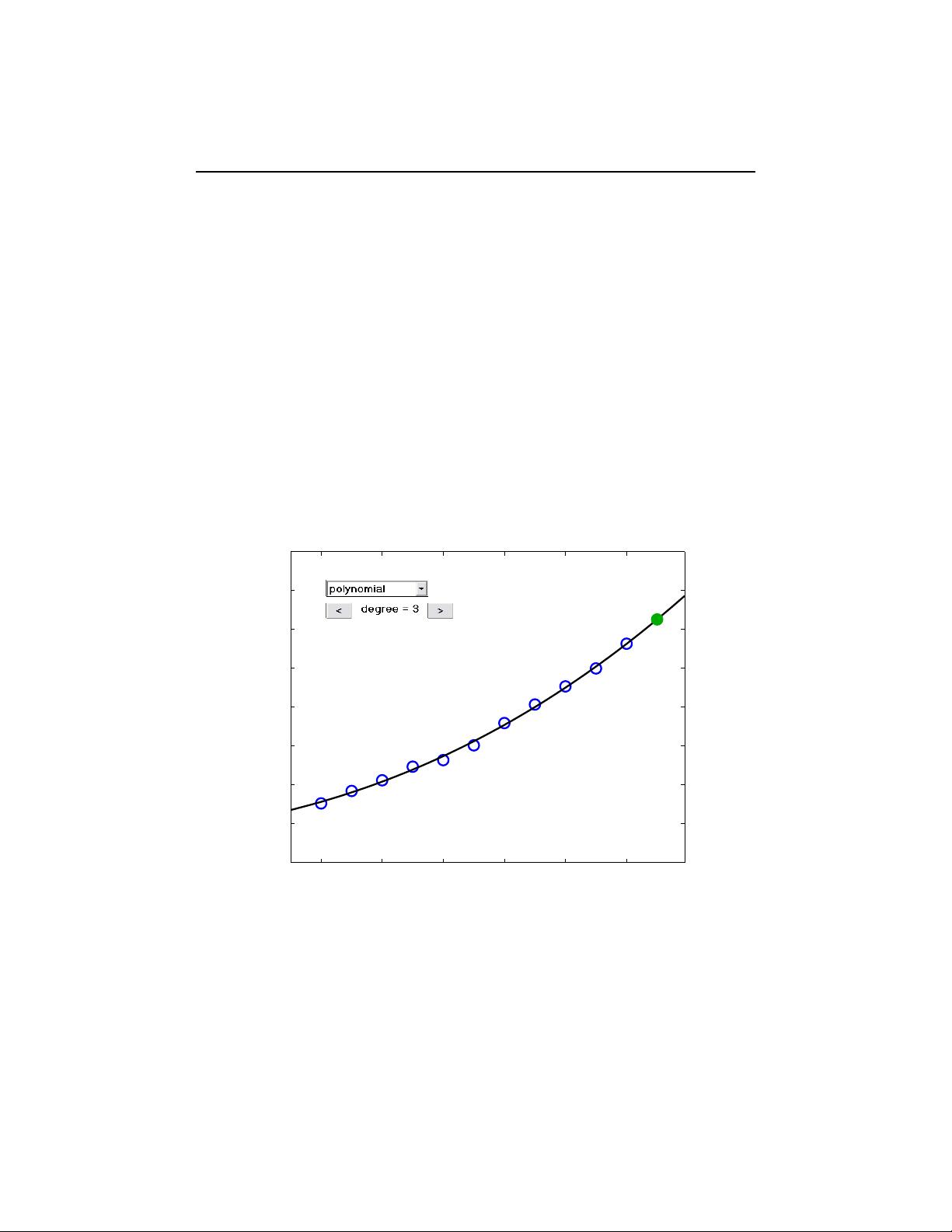
A very common source of least squares problems is curve fitting. Let t be the
independent variable and let y(t) denote an unknown function of t that we want
to approximate. Assume there are m observations, i.e. values of y measured at
specified values of t.
y
i
= y(t
i
), i = 1, . . . , m
The idea is to model y(t) by a linear combination of n basis functions,
y(t) ≈ β
1
φ
1
(t) + . . . + β
n
φ
n
(t)
The design matrix X is a rectangular matrix of order m-by-n with elements
x
i,j
= φ
j
(t
i
)
The design matrix usually has more rows than columns. In matrix-vector notation,
the model is
y ≈ Xβ
1
2 Chapter 5. Least Squares
The symbol ≈ stands for “is approximately equal to.” We are more precise about
this in the next section, but our emphasis is on least squares approximation.
The basis functions φ
j
(t) can be nonlinear functions of t, but the unknown
parameters, β
j
, appear in the model linearly. The system of linear equations
Xβ ≈ y
is overdetermined if there are more equations than unknowns. The Matlab back-
slash operator computes a least squares solution to such a system.
beta = X\y
The basis functions might also involve some nonlinear parameters, α
1
, . . . , α
p
.
The problem is separable if it involves both linear and nonlinear parameters.
y(t) ≈ β
1
φ
1
(t, α) + . . . + β
n
φ
n
(t, α)
The elements of the design matrix depend upon both t and α.
x
i,j
= φ
j
(t
i
, α)
Separable problems can be solved by combining backslash with the Matlab func-
tion fminsearch or one of the nonlinear minimizers available in the Optimization
Toolbox. The new Curve Fitting Toolbox provides a graphical interface for solving
nonlinear fitting problems.
Some common models include:
• Straight line: If the model is also linear in t, it is a straight line.
y(t) ≈ β
1
t + β
2
• Polynomials: The coefficients β
j
appear linearly. Matlab orders polynomials
with the highest power first.
φ
j
(t) = t
n−j
, j = 1, . . . , n
y(t) ≈ β
1
t
n−1
+ . . . + β
n−1
t + β
n
The Matlab function polyfit computes least squares polynomial fits by
setting up the design matrix and using backslash to find the coefficients.
• Rational functions: The coefficients in the numerator appear linearly; the
coefficients in the denominator appear nonlinearly.
φ
j
(t) =
t
n−j
α
1
t
n−1
+ . . . + α
n−1
t + α
n
y(t) ≈
β
1
t
n−1
+ . . . + β
n−1
t + β
n
α
1
t
n−1
+ . . . + α
n−1
t + α
n
5.2. Norms 3
• Exponentials: The decay rates, λ
j
, appear nonlinearly.
φ
j
(t) = e
−λ
j
t
y(t) ≈ β
1
e
−λ
1
t
+ . . . + β
n
e
−λ
n
t
• Log-linear: If there is only one exponential, taking logs makes the model
linear, but changes the fit criterion.
y(t) ≈ Ke
λt
log y ≈ β
1
t + β
2
, with β
1
= λ, β
2
= log K
• Gaussians: The means and variances appear nonlinearly.
φ
j
(t) = e
−
³
t−µ
j
σ
j
´
2
y(t) ≈ β
1
e
−
¡
t−µ
1
σ
1
¢
2
+ . . . β
n
e
−
(
t−µ
n
σ
n
)
2
5.2 Norms
The residuals are the differences between the observations and the model,
r
i
= y
i
−
n
X
1
β
j
φ
j
(t
i
, α), i = 1, . . . , m
Or, in matrix-vector notation,
r = y − X(α)β
We want to find the α’s and β’s that make the residuals as small as possible.
What do we mean by “small”? In other words, what do we mean when we use the
“≈” symbol? There are several possibilities.
• Interpolation: If the number of parameters is equal to the number of obser-
vations, we might be able to make the residuals zero. For linear problems,
this will mean that m = n and that the design matrix X is square. If X is
nonsingular, the β’s are the solution to a square system of linear equations.
β = X\y
• Least squares: Minimize the sum of the squares of the residuals.
krk
2
=
m
X
1
r
2
i
4 Chapter 5. Least Squares
• Weighted least squares: If some observations are more important or more
accurate than others, then we might associate different weights, w
j
, with
different observations and minimize
krk
2
w
=
m
X
1
w
i
r
2
i
For example, if the error in the ith observation is approximately e
i
, then
choose w
i
= 1/e
i
.
Any algorithm for solving an unweighted least squares problem can be used
to solve a weighted problem by scaling the observations and design matrix.
We simply multiply both y
i
and the ith row of X by w
i
. In Matlab, this
can be accomplished with
X = diag(w)*X
y = diag(w)*y
• One-norm: Minimize the sum of the absolute values of the residuals.
krk
1
=
m
X
1
|r
i
|
This problem can be reformulated as a linear programming problem, but it is
computationally more difficult than least squares. The resulting parameters
are less sensitive to the presence of spurious data points or outliers. .
• Infinity-norm: Minimize the largest residual.
krk
∞
= max
i
|r
i
|
This is also known as a Chebyshev fit and can be reformulated as a linear
programming problem. Chebyshev fits are frequently used in the design of
digital filters and in the development of approximations for use in mathemat-
ical function libraries.
The Matlab Optimization and Curve Fitting toolboxes include functions for
one-norm and infinity-norm problems. We will limit ourselves to least squares in
this book.
5.3 censusgui
The NCM program censusgui involves several different linear models. The data is
the total population of the United States, as determined by the U. S. Census, for
the years 1900 to 2000. The units are millions of people.
5.3. censusgui 5
t y
1900 75.995
1910 91.972
1900 105.711
1930 123.203
1940 131.669
1950 150.697
1960 179.323
1970 203.212
1980 226.505
1990 249.633
2000 281.422
The task is to mo del the population growth and predict the population when t =
2010. The default model in censusgui is a cubic polynomial in t.
y ≈ β
1
t
3
+ β
2
t
2
+ β
3
t + β
4
There are four unknown coefficients, appearing linearly.
1900 1920 1940 1960 1980 2000
0
50
100
150
200
250
300
350
400
Predict U.S. Population in 2010
Millions
312.691
Figure 5.1. censusgui
Numerically, it’s a bad idea to use powers of t as basis functions when t is
around 1900 or 2000. The design matrix is badly scaled and its columns are nearly
linearly dependent. A much better basis is provided by powers of a translated and
scaled t,
s = (t − 1950)/50
剩余26页未读,继续阅读
zxjnttc
- 粉丝: 0
- 资源: 7
上传资源 快速赚钱
- 我的内容管理 展开
- 我的资源 快来上传第一个资源
- 我的收益 登录查看自己的收益
- 我的积分 登录查看自己的积分
- 我的C币 登录后查看C币余额
- 我的收藏
- 我的下载
- 下载帮助
安全验证
文档复制为VIP权益,开通VIP直接复制
信息提交成功
评论0