export_fig
==========
A toolbox for exporting figures from MATLAB to standard image and document formats nicely.
### Overview
Exporting a figure from MATLAB the way you want it (hopefully the way it looks on screen), can be a real headache for the unitiated, thanks to all the settings that are required, and also due to some eccentricities (a.k.a. features and bugs) of functions such as `print`. The first goal of export_fig is to make transferring a plot from screen to document, just the way you expect (again, assuming that's as it appears on screen), a doddle.
The second goal is to make the output media suitable for publication, allowing you to publish your results in the full glory that you originally intended. This includes embedding fonts, setting image compression levels (including lossless), anti-aliasing, cropping, setting the colourspace, alpha-blending and getting the right resolution.
Perhaps the best way to demonstrate what export_fig can do is with some examples.
### Examples
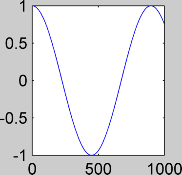
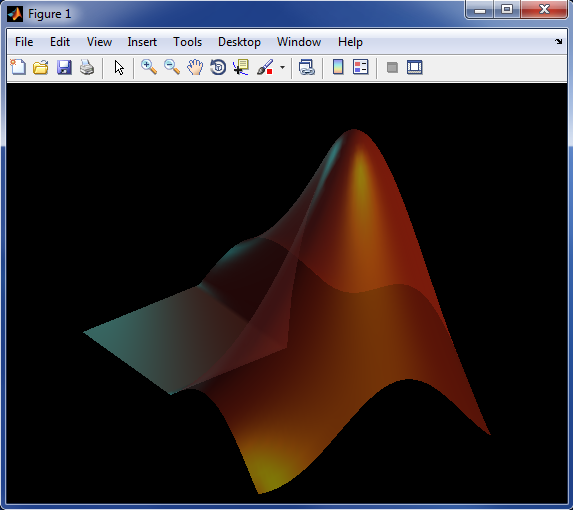
**Visual accuracy** - MATLAB's exporting functions, namely `saveas` and `print`, change many visual properties of a figure, such as size, axes limits and ticks, and background colour, in unexpected and unintended ways. Export_fig aims to faithfully reproduce the figure as it appears on screen. For example:
```Matlab
plot(cos(linspace(0, 7, 1000)));
set(gcf, 'Position', [100 100 150 150]);
saveas(gcf, 'test.png');
export_fig test2.png
```
generates the following:
| Figure: | test.png: | test2.png: |
|:-------:|:---------:|:----------:|
|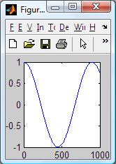|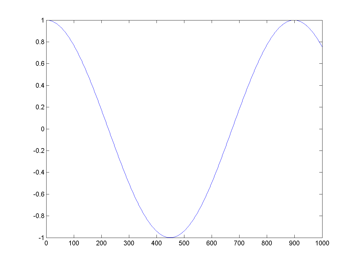|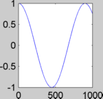|
Note that the size and background colour of test2.png (the output of export_fig) are the same as those of the on screen figure, in contrast to test.png. Of course, if you want the figure background to be white (or any other colour) in the exported file then you can set this prior to exporting using:
```Matlab
set(gcf, 'Color', 'w');
```
Notice also that export_fig crops and anti-aliases (smooths, for bitmaps only) the output by default. However, these options can be disabled; see the Tips section below for details.
**Resolution** - by default, export_fig exports bitmaps at screen resolution. However, you may wish to save them at a different resolution. You can do this using either of two options: `-m<val>`, where <val> is a positive real number, magnifies the figure by the factor <val> for export, e.g. `-m2` produces an image double the size (in pixels) of the on screen figure; `-r<val>`, again where <val> is a positive real number, specifies the output bitmap to have <val> pixels per inch, the dimensions of the figure (in inches) being those of the on screen figure. For example, using:
```Matlab
export_fig test.png -m2.5
```
on the figure from the example above generates:
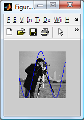
Sometimes you might have a figure with an image in. For example:
```Matlab
imshow(imread('cameraman.tif'))
hold on
plot(0:255, sin(linspace(0, 10, 256))*127+128);
set(gcf, 'Position', [100 100 150 150]);
```
generates this figure:
Here the image is displayed in the figure at resolution lower than its native resolution. However, you might want to export the figure at a resolution such that the image is output at its native (i.e. original) size (in pixels). Ordinarily this would require some non-trivial computation to work out what that resolution should be, but export_fig has an option to do this for you. Using:
```Matlab
export_fig test.png -native
```
produces:
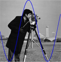
with the image being the size (in pixels) of the original image. Note that if you want an image to be a particular size, in pixels, in the output (other than its original size) then you can resize it to this size and use the `-native` option to achieve this.
All resolution options (`-m<val>`, `-q<val>` and `-native`) correctly set the resolution information in PNG and TIFF files, as if the image were the dimensions of the on screen figure.
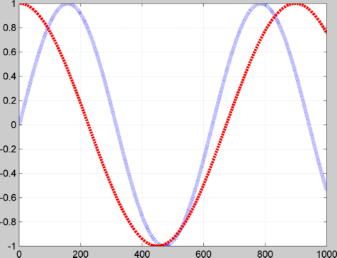
**Shrinking dots & dashes** - when exporting figures with dashed or dotted lines using either the ZBuffer or OpenGL (default for bitmaps) renderers, the dots and dashes can appear much shorter, even non-existent, in the output file, especially if the lines are thick and/or the resolution is high. For example:
```Matlab
plot(sin(linspace(0, 10, 1000)), 'b:', 'LineWidth', 4);
hold on
plot(cos(linspace(0, 7, 1000)), 'r--', 'LineWidth', 3);
grid on
export_fig test.png
```
generates:
This problem can be overcome by using the painters renderer. For example:
```Matlab
export_fig test.png -painters
```
used on the same figure generates:
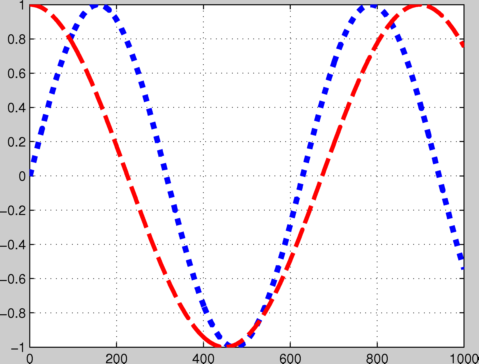
Note that not only are the plot lines correct, but the grid lines are too.
**Transparency** - sometimes you might want a figure and axes' backgrounds to be transparent, so that you can see through them to a document (for example a presentation slide, with coloured or textured background) that the exported figure is placed in. To achieve this, first (optionally) set the axes' colour to 'none' prior to exporting, using:
```Matlab
set(gca, 'Color', 'none'); % Sets axes background
```
then use export_fig's `-transparent` option when exporting:
```Matlab
export_fig test.png -transparent
```
This will make the background transparent in PDF, EPS and PNG outputs. You can additionally save fully alpha-blended semi-transparent patch objects to the PNG format. For example:
```Matlab
logo;
alpha(0.5);
```
generates a figure like this:
If you then export this to PNG using the `-transparent` option you can then put the resulting image into, for example, a presentation slide with fancy, textured background, like so:
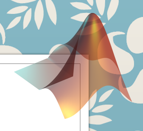
and the image blends seamlessly with the background.
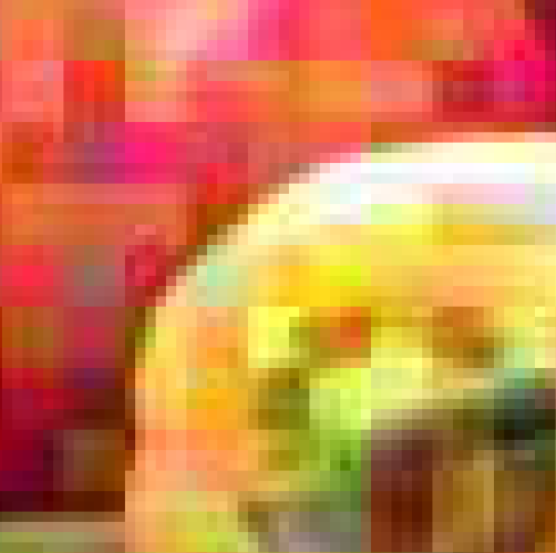
**Image quality** - when publishing images of your results, you want them to look as good as possible. By default, when outputting to lossy file formats (PDF, EPS and JPEG), export_fig uses a high quality setting, i.e. low compression, for images, so little information is lost. This is in contrast to MATLAB's print and saveas functions, whose default quality settings are poor. For example:
```Matlab
A = im2double(imread('peppers.png'));
B = randn(ceil(size(A, 1)/6), ceil(size(A, 2)/6), 3) * 0.1;
B = cat(3, kron(B(:,:,1), ones(6)), kron(B(:,:,2), ones(6)), kron(B(:,:,3), ones(6)));
B = A + B(1:size(A, 1),1:size(A, 2),:);
imshow(B);
print -dpdf test.pdf
```
generates a PDF file, a sub-window of which looks (when zoomed in) like this:
while the command
```Matlab
export_fig test.pdf
```
on the same figure produces this:
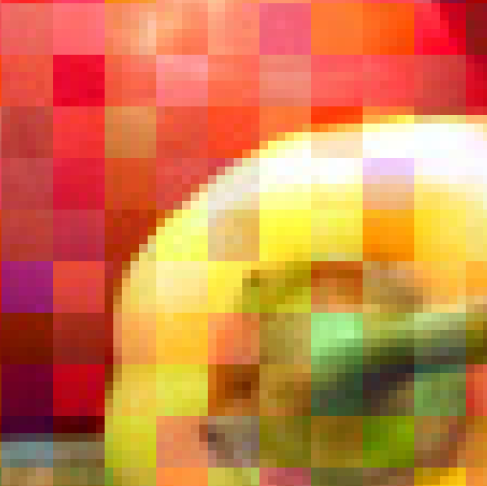
While much better, the image still contains some compression artifacts (see the low level noise around the edge of the pepper). You may prefer to export with no artifacts at all, i.e. lossless compression. Alternatively, you might need a smaller file, and be willing to accept more compression. Either way, export_fig has an option that can suit your needs: `-q<val>`, where <val> is a number from 0-100, will set the level of lossy image compression (again in PDF, EPS and JPEG outputs only; other formats are lossless), from high compression (0) to low compression/high quality (100). If you want lossless compression in any of those formats then specify a <val> greater than 100. For examp
用于Matlab的各种点云工具.zip

42 浏览量
2024-03-23
14:48:46
上传
评论
收藏 24.44MB ZIP 举报
 用于Matlab的各种点云工具.zip (216个子文件)
  CITATION.cff 478B ImageSelection.class 1KB
 icon_rgb.gif 890B icon_bypc.gif 889B icon_show_all.gif 875B icon_histo.gif 872B icon_save_screenshot.gif 871B icon_choose_limits.gif 869B icon_select_profile.gif 868B icon_set_limits.gif 866B icon_zoom_out.gif 863B icon_select_inpolygon.gif 861B icon_attributex.gif 861B icon_print_parameter.gif 860B icon_attributey.gif 859B icon_options.gif 859B icon_viewxz.gif 856B icon_viewxy.gif 856B icon_attributez.gif 856B icon_viewyz.gif 855B icon_toggle_axis.gif 855B icon_markersize10.gif 844B icon_markersize5.gif 841B icon_markersize1.gif 835B .gitattributes 378B .gitignore 2KB ImageSelection.java 1016B settings.json 30B LICENSE 1KB export_fig.m 57KB select.m 40KB solve.m 28KB plot_createToolbar.m 27KB print2eps.m 25KB ICP.m 19KB export.m 14KB msg.m 13KB pointCloud.m 13KB runICPMinimization.m 13KB runICP.m 11KB pcread.m 11KB print2array.m 9KB eps2pdf.m 8KB conAffPoint2PlaneSimpleOLS.m 8KB ghostscript.m 8KB plot_createMenu.m 7KB fix_lines.m 6KB conSimPoint2PlaneOLS.m 6KB im2gif.m 6KB runcmd.m 6KB plot_updatePlot.m 5KB getVoxelHull.m 5KB normals.m 5KB plotPolar.m 5KB isolate_axes.m 5KB createRaster.m 5KB transform.m 5KB crop_borders.m 5KB runICPInit.m 4KB plot_updateMenus.m 4KB globalICP.m 4KB corrPoints.m 4KB segmentation.m 4KB addPrm.m 4KB pdftops.m 3KB user_string.m 3KB plot.m 3KB runICPStats.m 3KB addAttribute.m 3KB xyz2polar.m 3KB runICPPlot.m 3KB scatter3ext.m 3KB plot_selectLimits.m 3KB plot_setPrmAndPlot.m 3KB assignIdxAdj.m 3KB alphashape.m 3KB img.m 3KB uniformSampling.m 3KB append_pdfs.m 3KB runICPSelection.m 3KB rejection.m 3KB runICPPairList.m 2KB dirext.m 2KB copy.m 2KB ecef2mapTrafo.m 2KB map2ecefTrafo.m 2KB addPC.m 2KB addObs.m 2KB transform.m 2KB plot_updateHisto.m 2KB info.m 2KB polyMesh.m 2KB plot_selectInPolygon.m 2KB importOri.m 2KB plotNormals.m 2KB match.m 2KB plot_selectProfile.m 2KB plot_showPointInfo.m 2KB runICPSaveResults.m 2KB getPrmCstObs.m 2KB
共 216 条
- 1
- 2
- 3
资源评论


若明天不见
- 粉丝: 1w+
- 资源: 273


最新资源
- 论文(最终)_20240430235101.pdf
- 基于python编写的Keras深度学习框架开发,利用卷积神经网络CNN,快速识别图片并进行分类
- 最全空间计量实证方法(空间杜宾模型和检验以及结果解释文档).txt
- 5uonly.apk
- 蓝桥杯Python组的历年真题
- 2023-04-06-项目笔记 - 第一百十九阶段 - 4.4.2.117全局变量的作用域-117 -2024.04.30
- 2023-04-06-项目笔记 - 第一百十九阶段 - 4.4.2.117全局变量的作用域-117 -2024.04.30
- 前端开发技术实验报告:内含4四实验&实验报告
- Highlight Plus v20.0.1
- 林周瑜-论文.docx
资源上传下载、课程学习等过程中有任何疑问或建议,欢迎提出宝贵意见哦~我们会及时处理!
点击此处反馈


