export_fig
==========
A toolbox for exporting figures from MATLAB to standard image and document formats nicely.
### Overview
Exporting a figure from MATLAB the way you want it (hopefully the way it looks on screen), can be a real headache for the unitiated, thanks to all the settings that are required, and also due to some eccentricities (a.k.a. features and bugs) of functions such as `print`. The first goal of export_fig is to make transferring a plot from screen to document, just the way you expect (again, assuming that's as it appears on screen), a doddle.
The second goal is to make the output media suitable for publication, allowing you to publish your results in the full glory that you originally intended. This includes embedding fonts, setting image compression levels (including lossless), anti-aliasing, cropping, setting the colourspace, alpha-blending and getting the right resolution.
Perhaps the best way to demonstrate what export_fig can do is with some examples.
### Examples
**Visual accuracy** - MATLAB's exporting functions, namely `saveas` and `print`, change many visual properties of a figure, such as size, axes limits and ticks, and background colour, in unexpected and unintended ways. Export_fig aims to faithfully reproduce the figure as it appears on screen. For example:
```Matlab
plot(cos(linspace(0, 7, 1000)));
set(gcf, 'Position', [100 100 150 150]);
saveas(gcf, 'test.png');
export_fig test2.png
```
generates the following:
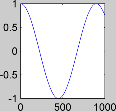
| Figure: | test.png: | test2.png: |
|:-------:|:---------:|:----------:|
|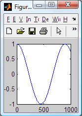|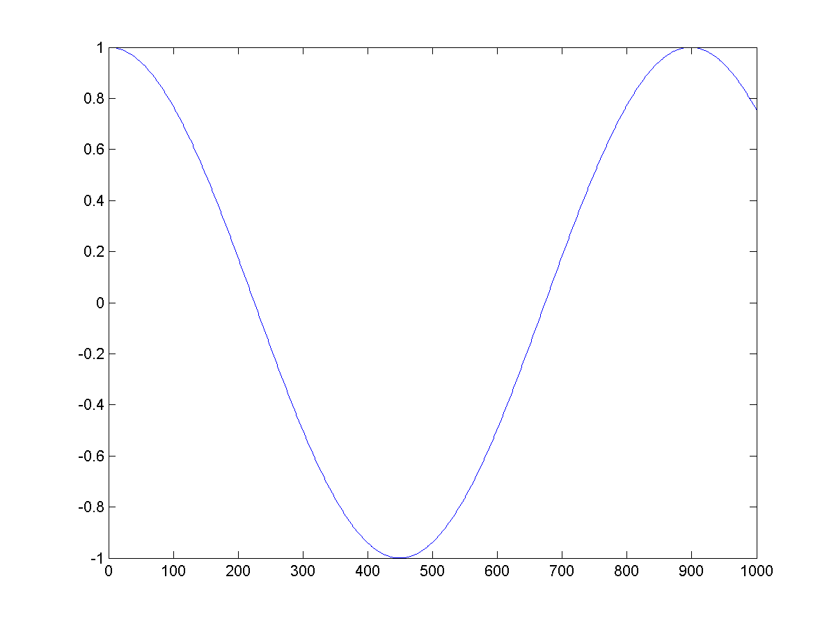|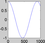|
Note that the size and background colour of test2.png (the output of export_fig) are the same as those of the on screen figure, in contrast to test.png. Of course, if you want the figure background to be white (or any other colour) in the exported file then you can set this prior to exporting using:
```Matlab
set(gcf, 'Color', 'w');
```
Notice also that export_fig crops and anti-aliases (smooths, for bitmaps only) the output by default. However, these options can be disabled; see the Tips section below for details.
**Resolution** - by default, export_fig exports bitmaps at screen resolution. However, you may wish to save them at a different resolution. You can do this using either of two options: `-m<val>`, where <val> is a positive real number, magnifies the figure by the factor <val> for export, e.g. `-m2` produces an image double the size (in pixels) of the on screen figure; `-r<val>`, again where <val> is a positive real number, specifies the output bitmap to have <val> pixels per inch, the dimensions of the figure (in inches) being those of the on screen figure. For example, using:
```Matlab
export_fig test.png -m2.5
```
on the figure from the example above generates:
Sometimes you might have a figure with an image in. For example:
```Matlab
imshow(imread('cameraman.tif'))
hold on
plot(0:255, sin(linspace(0, 10, 256))*127+128);
set(gcf, 'Position', [100 100 150 150]);
```
generates this figure:
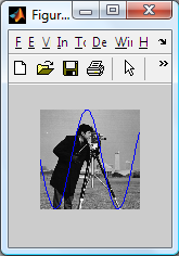
Here the image is displayed in the figure at resolution lower than its native resolution. However, you might want to export the figure at a resolution such that the image is output at its native (i.e. original) size (in pixels). Ordinarily this would require some non-trivial computation to work out what that resolution should be, but export_fig has an option to do this for you. Using:
```Matlab
export_fig test.png -native
```
produces:
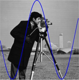
with the image being the size (in pixels) of the original image. Note that if you want an image to be a particular size, in pixels, in the output (other than its original size) then you can resize it to this size and use the `-native` option to achieve this.
All resolution options (`-m<val>`, `-q<val>` and `-native`) correctly set the resolution information in PNG and TIFF files, as if the image were the dimensions of the on screen figure.
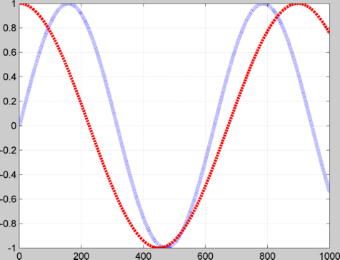
**Shrinking dots & dashes** - when exporting figures with dashed or dotted lines using either the ZBuffer or OpenGL (default for bitmaps) renderers, the dots and dashes can appear much shorter, even non-existent, in the output file, especially if the lines are thick and/or the resolution is high. For example:
```Matlab
plot(sin(linspace(0, 10, 1000)), 'b:', 'LineWidth', 4);
hold on
plot(cos(linspace(0, 7, 1000)), 'r--', 'LineWidth', 3);
grid on
export_fig test.png
```
generates:
This problem can be overcome by using the painters renderer. For example:
```Matlab
export_fig test.png -painters
```
used on the same figure generates:
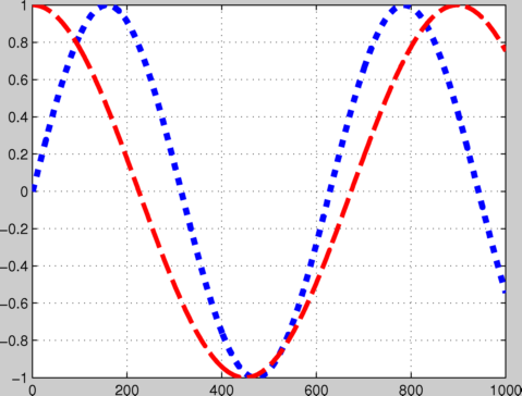
Note that not only are the plot lines correct, but the grid lines are too.
**Transparency** - sometimes you might want a figure and axes' backgrounds to be transparent, so that you can see through them to a document (for example a presentation slide, with coloured or textured background) that the exported figure is placed in. To achieve this, first (optionally) set the axes' colour to 'none' prior to exporting, using:
```Matlab
set(gca, 'Color', 'none'); % Sets axes background
```
then use export_fig's `-transparent` option when exporting:
```Matlab
export_fig test.png -transparent
```
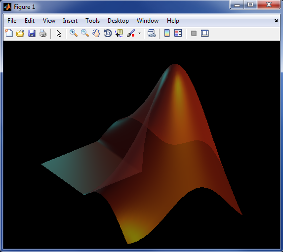
This will make the background transparent in PDF, EPS and PNG outputs. You can additionally save fully alpha-blended semi-transparent patch objects to the PNG format. For example:
```Matlab
logo;
alpha(0.5);
```
generates a figure like this:
If you then export this to PNG using the `-transparent` option you can then put the resulting image into, for example, a presentation slide with fancy, textured background, like so:
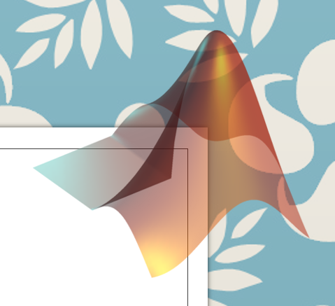
and the image blends seamlessly with the background.
**Image quality** - when publishing images of your results, you want them to look as good as possible. By default, when outputting to lossy file formats (PDF, EPS and JPEG), export_fig uses a high quality setting, i.e. low compression, for images, so little information is lost. This is in contrast to MATLAB's print and saveas functions, whose default quality settings are poor. For example:
```Matlab
A = im2double(imread('peppers.png'));
B = randn(ceil(size(A, 1)/6), ceil(size(A, 2)/6), 3) * 0.1;
B = cat(3, kron(B(:,:,1), ones(6)), kron(B(:,:,2), ones(6)), kron(B(:,:,3), ones(6)));
B = A + B(1:size(A, 1),1:size(A, 2),:);
imshow(B);
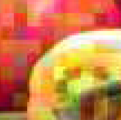
print -dpdf test.pdf
```
generates a PDF file, a sub-window of which looks (when zoomed in) like this:
while the command
```Matlab
export_fig test.pdf
```
on the same figure produces this:
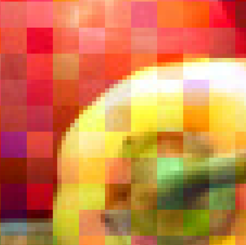
While much better, the image still contains some compression artifacts (see the low level noise around the edge of the pepper). You may prefer to export with no artifacts at all, i.e. lossless compression. Alternatively, you might need a smaller file, and be willing to accept more compression. Either way, export_fig has an option that can suit your needs: `-q<val>`, where <val> is a number from 0-100, will set the level of lossy image compression (again in PDF, EPS and JPEG outputs only; other formats are lossless), from high compression (0) to low compression/high quality (100). If you want lossless compression in any of those formats then specify a <val> greater than 100. For examp
滑移分析工具箱和GUI ( Matlab )(高分项目).zip

需积分: 3 62 浏览量
2024-03-09
15:15:20
上传
评论
收藏 43.06MB ZIP 举报
 滑移分析工具箱和GUI ( Matlab )(高分项目).zip (672个子文件)
  validation1_AngFile(forMTEX).ang 10.78MB validation1_AngFile(forMTEX)_2phases.ang 9.31MB b12_scan01.ang 2.69MB b12_scan02.ang 2.69MB b12_scan03.ang 2.69MB b12_scan04.ang 2.69MB b12_scan05.ang 2.69MB b12_scan06.ang 2.69MB b12_scan08.ang 2.69MB b12_scan07.ang 2.69MB make.bat 6KB slip_transmission_BX_refs.bib 12KB
 logo_MPIE_MSU.bmp 293KB Tialpha.cif 2KB ImageSelection.class 1KB ImageSelection.class 1KB theme_overrides.css 39B exampleHKL.ctf 37.82MB
 STABiX_ebsdmap.gif 4.49MB gui_gb_inc.png.gif 1.55MB .gitignore 205B .gitignore 120B .gitignore 31B .gitignore 6B
 selftest_report.html 3KB selftest_report.html 3KB README.html 233B
 snakeyaml-1.9.jar 260KB ImageSelection.java 1016B ImageSelection.java 1016B
 EBSDmap.jpg 183KB LICENSE 34KB LICENSE 1KB arrow.m 54KB export_fig.m 53KB screencapture.m 34KB preCPFE_indentation_setting_BX.m 27KB interface_map_plotmap.m 23KB print2eps.m 19KB slip_systems.m 19KB interface_map_mprime_calculator_map.m 18KB A_gui_plotmap.m 17KB interface_map_plotmap_nodata.m 13KB align_crop_3DEBSD_dataset.m 13KB listLattParam.m 12KB A_gui_plotGB_Bicrystal.m 12KB plotGB_Bicrystal.m 12KB plotGB_Bicrystal_mprime_calculator_bc.m 12KB vis_hex.m 11KB preCPFE_indentation_setting_SX.m 10KB xticklabel_rotate.m 10KB listElasticConstants.m 10KB plotGB_Bicrystal_mprime_calculator_all.m 10KB DateTime.m 10KB print2array.m 9KB write_oim_ang_file_v7.m 9KB write_oim_ang_file_v6.m 9KB test_ReadYaml.m 9KB vis_bcc.m 8KB plotGB_Bicrystal_load_YAML_config_file.m 8KB interface_map_init_microstructure.m 8KB plotGB_Bicrystal_max_min_values_from_matrix.m 8KB diverging_map.m 8KB preCPFE_set_valid_inputs_BX.m 8KB plotGB_Bicrystal_gbax_title_and_text.m 8KB ReadYamlRaw.m 8KB eps2pdf.m 7KB preCPFE_load_mesh.m 7KB Kehiagas1995_all_rbv_plot_noYAML.m 7KB ghostscript.m 7KB preCPFE_generate_indentation_model_BX.m 7KB vis_fcc.m 7KB A_gui_gbinc.m 7KB Kacher2012_1_plot.m 7KB parula.m 7KB preCPFE_generate_indentation_model_SX.m 7KB WriteYaml.m 7KB preCPFE_set_valid_inputs_SX.m 6KB fix_lines.m 6KB plotGB_Bicrystal_update_slip.m 6KB write_hkl_ctf_file.m 6KB im2gif.m 6KB interface_map_screenshots.m 6KB A_preCPFE_windows_indentation_setting_BX.m 6KB MTEX2016_Mercier_1st_exercise_final.m 6KB write_oim_grain_file_type2.m 6KB write_oim_reconstructed_boundaries_file.m 6KB interface_map_read_TSL_data.m 6KB Kacher2014_all_rbv_plot_noYAML.m 6KB plotGB_Bicrystal_plot_lattices.m 5KB makematrices.m 5KB preCPFE_buttons_indenter.m 5KB mtex_convert2TSLdata.m 5KB mergeimports.m 5KB demo.m 5KB MTEX2016_Mercier_3rd_exercise_final.m 5KB preCPFE_load_YAML_BX_config_file.m 5KB read_oim_reconstructed_boundaries_file.m 5KB catstruct.m 5KB read_oim_grain_file_type2.m 5KB
共 672 条
- 1
- 2
- 3
- 4
- 5
- 6
- 7
资源评论


