Path Planning for Autonomous Vehicles in Unknown Semi-structured

Dmitri Dolgov

AI & Robotics Group,

Toyota Research Institute,

Ann Arbor, MI 48105,

USA

ddolgov@ai.stanford.edu

Sebastian Thrun

Michael Montemerlo

James Diebel

Environments

Abstract

We describe a practical path-planning algorithm for an autonomous

vehicle operating in an unknown semi-structured (or unstructured)

environment, where obstacles are detected online by the robot’s sen-

sors. This work was motivated by and experimentally validated in the

2007 DARPA Urban Challenge, where robotic vehicles had to au-

extend our algorithm to use prior topological knowledge of the envi-

ronment to guide path planning, leading to faster search and final tra-

jectories better suited to the structure of the environment. We present

experimental results from the DARPA Urban Challenge, where our

robot demonstrated near-flawless performance in complex general

path-planning tasks such as navigating parking lots and executing

U-turns on blocked roads. We also present results on autonomous

http://www.sagepub.co.uk/journalsPermissions.nav

Figures 1–15, 17 appear in color online: http://ijr.sagepub.com

KEY WORDS—path planning, autonomous driving

1. Introduction

The task of autonomous driving has received much attention

from the robotics community, especially in recent years with

events such as the DARPA Grand Challenges (Buehler et al.

2005) and the Urban Challenge (Buehler et al. 2008a,b) serv-

ing to catalyze research in the field.

In this paper, we focus on the problem of path planning

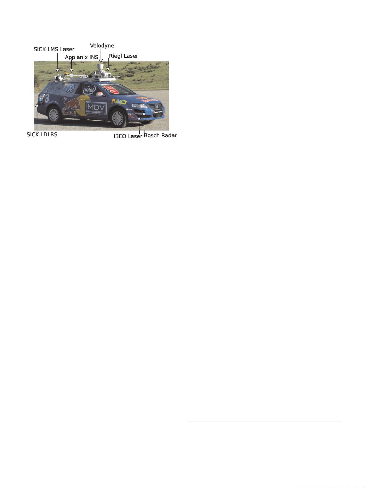
rithm described in this paper was used by the Stanford Racing

Team’s robot, Junior (Figure 1), in the DUC

space path-planning tasks (many involving driving in reverse)

such as navigating parking lots, executing U-turns, and dealing

with blocked intersections.

Fig. 1. Junior, our entry in the DUC. Junior is equipped with

several LIDAR and RADAR units, and a high-accuracy GPS

trols (and hence trajectories) is continuous, leading to a com-

plex, continuous-variable optimization problem. Much of the

20051 Nash et al. 2007) yields fast algorithms for discrete state

spaces, but those algorithms tend to produce paths that are non-

smooth and do not generally satisfy the non-holonomic con-

Another approach is to directly formulate the path-planning

problem as a non-linear optimization problem in the space of

controls or in the space of parametrized curves (Cremean et

al. 2006). However, in practice, guaranteeing fast convergence

Our path-planning algorithm builds on the existing work

discussed above and consists of two main phases. The first

phase uses a heuristic search in continuous coordinates to pro-

earlier versions of our path-planing work (Dolgov et al. 2008).

This two-phase approach to path planning works well in un-

structured environments (such as the “free-navigation zones”

in the DUC). However, this free-space planner often produces

trajectories that are not well suited to semi-structured environ-

ments, such as real parking lots. In situations where the envi-

ronment has strong topological structure, it is important for the

robot to observe that structure. For example, cutting across a

like our robotic vehicle (for the most part) to stay on the given

lane graph. However, just as human drivers do, the robot might

need to significantly deviate from the graph while performing

maneuvers such as turning around, pulling in and out of park-

ing spaces, avoiding other cars, etc.

In situations where a topological lane graph is available to

the robot, we extend the two phases of our path-planning algo-

rithm to take that prior information into account. The resulting

leading to a faster search and producing final trajectories that

one is the 3D LIDAR (Velodyne).

stacle map (in our implementation, a grid), an initial state of

cle, respectively. The desired output is a trajectory (sequence

distance cost. For example, in the situation shown in the top

row of Figure 3, a search with the Euclidean-distance heuris-

tic expands 20,790 nodes, while the non-holonomic-without-

obstacles heuristic expands 12,196 nodes. The heuristic is sen-

sitive to the density of obstacles in the environment. In rel-

atively densely populated environments, such as the ones in

Figure 3, the benefits are fairly small (a factor of two in Fig-

Challenge), we frequently obtained an order-of-magnitude im-

provement in the number of expanded nodes.

Fig. 3. Search heuristics. Euclidean 2D distance expands 20,790 nodes (a). The non-holonomic-without-obstacles heuristic is

better: it expands 12,196 nodes (b), but can lead to wasteful exploration of dead-ends in more complex settings (c), where it

expands 37,181 nodes. Combining the latter with the holonomic-with-obstacles heuristic leads to a search tree with 11,302 nodes

(d).

essence, given some path-cost function (e.g. collision avoid-

ance) imposed on the configuration space f

4D search away from these areas.

Since both heuristics are mathematically admissible in the

A* sense, the maximum of the two can be used. In the sce-

nario shown in the bottom row of Figure 3, a search using only

the first (non-holonomic-without-obstacles) heuristic expands

37,181 nodes, while a search that uses both heuristics expands

scribed above were also independently developed (for a

of control actions (steering). This means that the search will

never reach the exact continuous-coordinate goal state (the ac-

curacy depends on the resolution of the grid in A*). To ad-

we augment the search with analytic expansions based on the

Reed–Shepp model (Reeds and Shepp 1990). In the search de-

kinematic model of the car (using a particular control action)