

I
terative learning control (ILC) is based on the notion
that the performance of a system that executes the
same task multiple times can be improved by learning
from previous executions (trials, iterations, passes).
For instance, a basketball player shooting a free throw
from a fixed position can improve his or her ability to
score by practicing the shot repeatedly. During each shot,
the basketball player observes
the trajectory of the ball and
consciously plans an alteration
in the shooting motion for the
next attempt. As the player
continues to practice, the cor-
rect motion is learned and becomes ingrained into the
muscle memory so that the shooting accuracy is iteratively
improved. The converged muscle motion profile is an
open-loop control generated through repetition and learn-
ing. This type of learned open-loop control strategy is the
essence of ILC.
We consider learning controllers for systems that per-
form the same operation repeatedly and under the same
operating conditions. For such systems, a nonlearning con-
troller yields the same tracking error on each pass. Although
error signals from previous iterations are information rich,
they are unused by a nonlearning controller. The objective
of ILC is to improve performance by incorporating error
information into the control for subsequent iterations. In
doing so, high performance can be achieved with low tran-
sient tracking error despite large model uncertainty and
repeating disturbances.
ILC differs from other
learning-type control strate-
gies, such as adaptive control,
neural networks, and repeti-
tive control (RC). Adaptive
control strategies modify the controller, which is a system,
whereas ILC modifies the control input, which is a signal
[1]. Additionally, adaptive controllers typically do not take
advantage of the information contained in repetitive com-
mand signals. Similarly, neural network learning involves
the modification of controller parameters rather than a
control signal; in this case, large networks of nonlinear
neurons are modified. These large networks require exten-
sive training data, and fast convergence may be difficult to
DOUGLAS A. BRISTOW, MARINA THARAYIL,
and ANDREW G. ALLEYNE
A LEARNING-BASED METHOD
FOR HIGH-PERFORMANCE
TRACKING CONTROL
©DIGITALVISION & ARTVILLE
96 IEEE CONTROL SYSTEMS MAGAZINE » JUNE 2006 1066-033X/06/$20.00©2006IEEE
guarantee [2], whereas ILC usually converges adequately
in just a few iterations.
ILC is perhaps most similar to RC [3] except that RC is
intended for continuous operation, whereas ILC is intend-
ed for discontinuous operation. For example, an ILC appli-
cation might be to control a robot that performs a task,
returns to its home position, and comes to a rest before
repeating the task. On the other hand, an RC application
might be to control a hard disk drive’s read/write head, in
which each iteration is a full rotation of the disk, and the
next iteration immediately follows the current iteration.
The difference between RC and ILC is the setting of the ini-
tial conditions for each trial [4]. In ILC, the initial condi-
tions are set to the same value on each trial. In RC, the
initial conditions are set to the final conditions of the previ-
ous trial. The difference in initial-condition resetting leads
to different analysis techniques and results [4].
Traditionally, the focus of ILC has been on improving
the performance of systems that execute a single, repeated
operation. This focus includes many practical industrial
systems in manufacturing, robotics, and chemical process-
ing, where mass production on an assembly line entails
repetition. ILC has been successfully applied to industrial
robots [5]–[9], computer numerical control (CNC) machine
tools [10], wafer stage motion systems [11], injection-mold-
ing machines [12], [13], aluminum extruders [14], cold
rolling mills [15], induction motors [16], chain conveyor
systems [17], camless engine valves [18], autonomous vehi-
cles [19], antilock braking [20], rapid thermal processing
[21], [22], and semibatch chemical reactors [23].
ILC has also found application to systems that do not
have identical repetition. For instance, in [24] an underwa-
ter robot uses similar motions in all of its tasks but with
different task-dependent speeds. These motions are equal-
ized by a time-scale transformation, and a single ILC is
employed for all motions. ILC can also serve as a training
mechanism for open-loop control. This technique is used
in [25] for fast-indexed motion control of low-cost, highly
nonlinear actuators. As part of an identification procedure,
ILC is used in [26] to obtain the aerodynamic drag coeffi-
cient for a projectile. Finally, [27] proposes the use of ILC
to develop high-peak power microwave tubes.
The basic ideas of ILC can be found in a U.S. patent [28]
filed in 1967 as well as the 1978 journal publication [29]
written in Japanese. However, these ideas lay dormant
until a series of articles in 1984 [5], [30]–[32] sparked wide-
spread interest. Since then, the number of publications on
ILC has been growing rapidly, including two special issues
[33], [34], several books [1], [35]–[37], and two surveys [38],
[39], although these comparatively early surveys capture
only a fraction of the results available today.
As illustrated in “Iterative Learning Control Versus
Good Feedback and Feedforward Design,” ILC has clear
advantages for certain classes of problems but is not
applicable to every control scenario. The goal of the pre-
sent article is to provide a tutorial that gives a complete
picture of the benefits, limitations, and open problems of
ILC. This presentation is intended to provide the practic-
ing engineer with the ability to design and analyze a sim-
ple ILC as well as provide the reader with sufficient
background and understanding to enter the field. As such,
the primary, but not exclusive, focus of this survey is on
single-input, single-output (SISO) discrete-time linear sys-
tems. ILC results for this class of systems are accessible
without extensive mathematical definitions and deriva-
tions. Additionally, ILC designs using discrete-time
JUNE 2006 « IEEE CONTROL SYSTEMS MAGAZINE 97
Iterative Learning Control Versus Good
Feedback and Feedforward Design
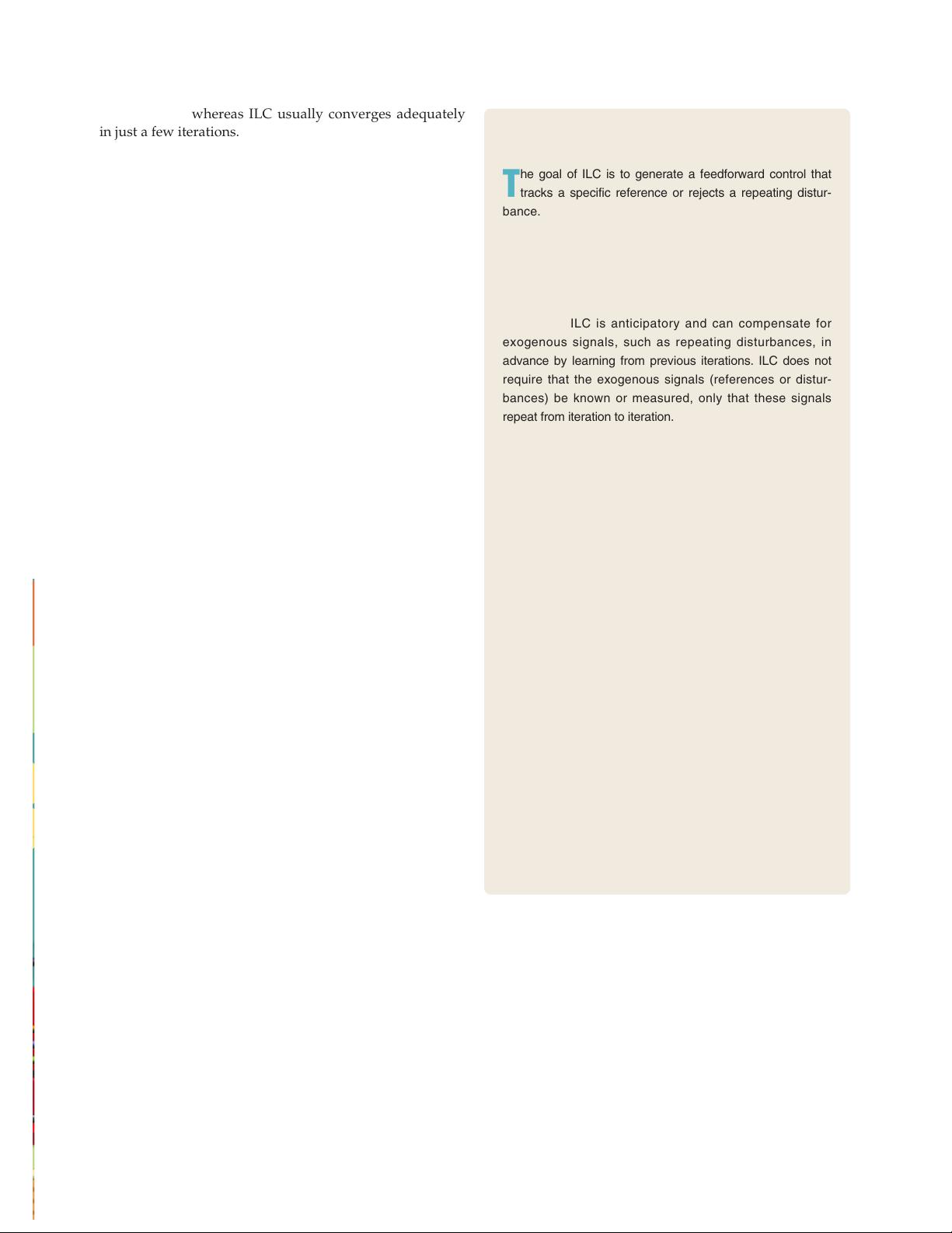
T
he goal of ILC is to generate a feedforward control that
tracks a specific reference or rejects a repeating distur-
bance. ILC has several advantages over a well-designed
feedback and feedforward controller. Foremost is that a feed-
back controller reacts to inputs and disturbances and, there-
fore, always has a lag in transient tracking. Feedforward
control can eliminate this lag, but only for known or measur-
able signals, such as the reference, and typically not for dis-
turbances. ILC is anticipatory and can compensate for
exogenous signals, such as repeating disturbances, in
advance by learning from previous iterations. ILC does not
require that the exogenous signals (references or distur-
bances) be known or measured, only that these signals
repeat from iteration to iteration.
While a feedback controller can accommodate variations
or uncertainties in the system model, a feedforward controller
performs well only to the extent that the system is accurately
known. Friction, unmodeled nonlinear behavior, and distur-
bances can limit the effectiveness of feedforward control.
Because ILC generates its open-loop control through prac-
tice (feedback in the iteration domain), this high-performance
control is also highly robust to system uncertainties. Indeed,
ILC is frequently designed assuming linear models and
applied to systems with nonlinearities yielding low tracking
errors, often on the order of the system resolution.
ILC cannot provide perfect tracking in every situation,
however. Most notably, noise and nonrepeating disturbances
hinder ILC performance. As with feedback control, observers
can be used to limit noise sensitivity, although only to the
extent to which the plant is known. However, unlike feedback
control, the iteration-to-iteration learning of ILC provides
opportunities for advanced filtering and signal processing.
For instance, zero-phase filtering [43], which is noncausal,
allows for high-frequency attenuation without introducing lag.
Note that these operations help to alleviate the sensitivity of
ILC to noise and nonrepeating disturbances. To reject nonre-
peating disturbances, a feedback controller used in combina-
tion with the ILC is the best approach.
linearizations of nonlinear systems often yield good results
when applied to the nonlinear systems [10], [22], [40]–[43].
ITERATIVE LEARNING CONTROL OVERVIEW
Linear Iterative Learning Control
System Description
Consider the discrete-time, linear time-invariant (LTI),
SISO system
y
j
(k) = P(q)u
j
(k) + d(k), (1)
where
k
is the time index,
j
is the iteration index,
q
is the
forward time-shift operator
qx(k) ≡ x(k +1)
,
y
j
is the out-
put,
u
j
is the control input, and
d
is an exogenous signal
that repeats each iteration. The plant
P(q)
is a proper ratio-
nal function of q and has a delay, or equivalently relative
degree, of
m
. We assume that
P(q)
is asymptotically stable.
When
P(q)
is not asymptotically stable, it can be stabilized
with a feedback controller, and the ILC can be applied to
the closed-loop system.
Next consider the
N
-sample sequence of inputs and
outputs
u
j
(k), k ∈{0, 1,...,N − 1},
y
j
(k), k ∈{m, m + 1,...,N + m −1},
d(k), k ∈{m, m +1,...,N + m − 1},
and the desired system output
y
d
(k), k ∈{m, m + 1,...,N + m −1}.
The performance or error signal is defined by
e
j
(k) = y
d
(k) − y
j
(k)
. In practice, the time duration
N
of the
trial is always finite, although sometimes it is useful for
analysis and design to consider an infinite time duration of
the trials [44]. In this work we use
N =∞
to denote trials with an infi-
nite time duration. The iteration
dimension indexed by
j
is usually
considered infinite with
j ∈{0, 1, 2,...}
. For simplicity in this
article, unless stated otherwise, the
plant delay is assumed to be
m = 1
.
Discrete time is the natural
domain for ILC because ILC explicit-
ly requires the storage of past-itera-
tion data, which is typically
sampled. System (1) is sufficiently
general to capture IIR [11] and FIR
[45] plants
P(q)
. Repeating distur-
bances [44], repeated nonzero initial
conditions [4], and systems aug-
mented with feedback and feedfor-
ward control [44] can be captured in
d(k)
. For instance, to incorporate the effect of repeated
nonzero initial conditions, consider the system
x
j
(k +1) = Ax
j
(k) + Bu
j
(k)(2)
y
j
(k) = Cx
j
(k), (3)
with
x
j
(0) = x
0
for all
j
. This state-space system is equiv-
alent to
y
j
(k) = C(qI − A)
−1
B
P(q)
u
j
(k) + CA
k
x
0
d(k)
.
Here, the signal
d(k)
is the free response of the system to
the initial condition
x
0
.
A widely used ILC learning algorithm [1], [35], [38] is
u
j+1
(k) = Q(q)[u
j
(k) + L(q)e
j
(k +1)],(4)
where the LTI dynamics
Q(q)
and
L(q)
are defined as the
Q-filter and learning function, respectively. The two-
dimensional (2-D) ILC system with plant dynamics (1) and
learning dynamics (4) is shown in Figure 1.
General Iterative Learning Control Algorithms
There are several possible variations to the learning algo-
rithm (4). Some researchers consider algorithms with lin-
ear time-varying (LTV) functions [42], [46], [47], nonlinear
functions [37], and iteration-varying functions [1], [48].
Additionally, the order of the algorithm, that is, the num-
ber
N
0
of previous iterations of
u
i
and
e
i
,
i ∈{j− N
0
+ 1,..., j}
, used to calculate
u
j+1
can be
increased. Algorithms with
N
0
> 1
are referred to as high-
er-order learning algorithms [26], [36], [37], [44], [49]–[51].
The current error
e
j+1
can also be used in calculating
u
j+1
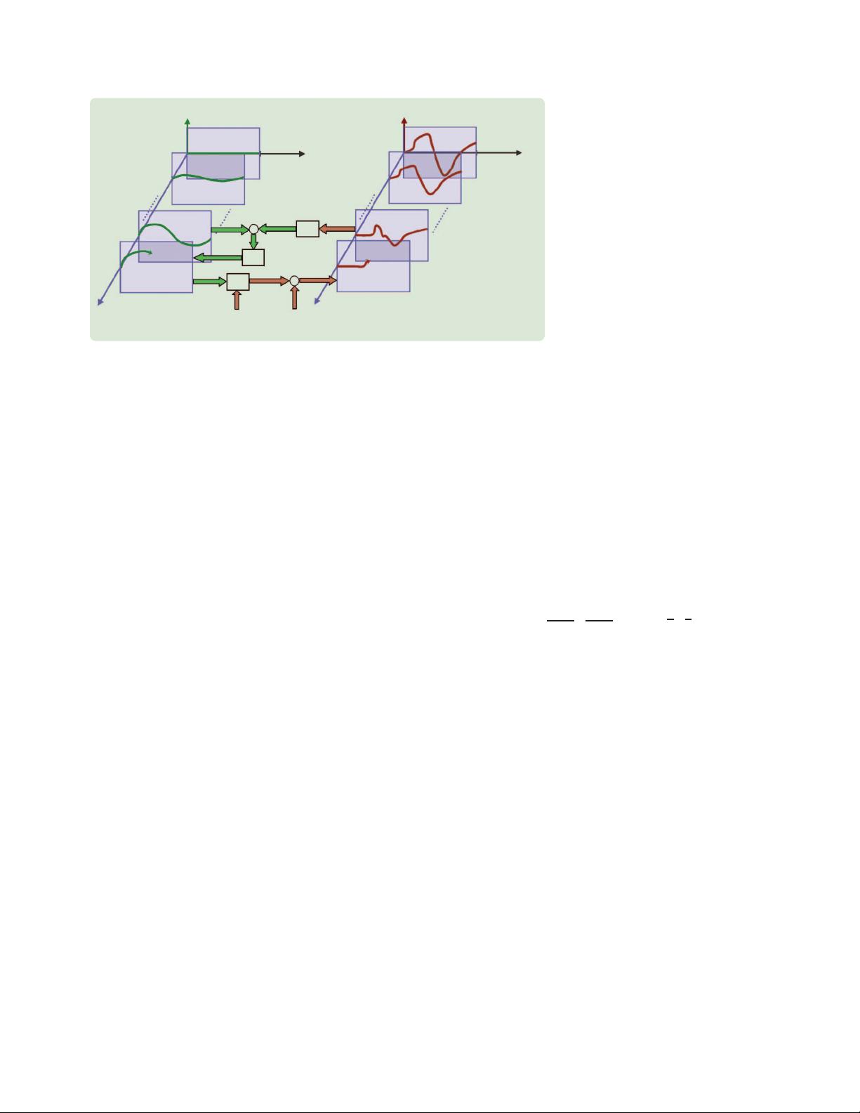
FIGURE 1 A two-dimensional, first-order ILC system. At the end of each iteration, the error is
filtered through L, added to the previous control, and filtered again through Q. This updated
open-loop control is applied to the plant in the next iteration.
Sample
Time
Sample
Time
j+1
j+1
jj
Iteration Iteration
1
0
1
0
0
Q
Control
Signal
L
P
Error
NN−1
1
++
+
−
Disturbance Reference
98 IEEE CONTROL SYSTEMS MAGAZINE » JUNE 2006
to obtain a current-iteration learning algorithm [52]–[56].
As shown in [57] and elsewhere in this article (see “Cur-
rent-Iteration Iterative Learning Control”), the current-iter-
ation learning algorithm is equivalent to the algorithm (4)
combined with a feedback controller on the plant.
Outline
The remainder of this article is divided into four major
sections. These are “System Representations,” “Analy-
sis,” “Design,” and “Implementation Example.” Time
and frequency-domain representations of the ILC sys-
tem are presented in the “System Representation” sec-
tion. The “Analysis” section examines the four basic
topics of greatest relevance to understanding ILC sys-
tem behavior: 1) stability, 2) performance, 3) transient
learning behavior, and 4) robustness. The “Design” sec-
tion investigates four different design methods: 1) PD
type, 2) plant inversion, 3)
H
∞
, and 4) quadratically
optimal. The goal is to give the reader an array of tools
to use and the knowledge of when each is appropriate.
Finally, the design and implementation of an iterative
learning controller for microscale robotic deposition
manufacturing is presented in the “Implementation
Example” section. This manufacturing example gives a
quantitative evaluation of ILC benefits.
SYSTEM REPRESENTATIONS
Analytical results for ILC systems are developed using two
system representations. Before proceeding with the analy-
sis, we introduce these representations.
Time-Domain Analysis Using the
Lifted-System Framework
To construct the lifted-system representation, the rational
LTI plant (1) is first expanded as an infinite power series
by dividing its denominator into its numerator, yielding
P(q) = p
1
q
−1
+ p
2
q
−2
+ p
3
q
−3
+ ···,(5)
where the coefficients
p
k
are Markov parameters [58].
The sequence
p
1
, p
2
,...
is the impulse response. Note
that
p
1
= 0
since
m = 1
is assumed. For the state space
description (2), (3),
p
k
is given by
p
k
= CA
k−1
B
. Stack-
ing the signals in vectors, the system dynamics in (1)
can be written equivalently as the
N × N
-dimensional
lifted system
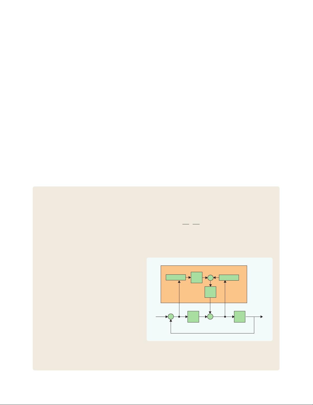
Current-Iteration Iterative Learning Control
C
urrent-iteration ILC is a method for incorporating feedback with ILC [52]–[56]. The current-iteration ILC
algorithm is given by
u
j+1
(k) = Q(q)[u
j
(k) + L(q)e
j
(k + 1)] + C(q)e
j+1
(k)
Feedback control
and shown in Figure A. This learning scheme derives its name from the addition of a learning component in the current iteration
through the term
C(q)e
j +1
(k)
. This algorithm, however, is identical to the algorithm (4) combined with a feedback controller in the
parallel architecture. Equivalence can be found between these two forms by separating the current-iteration ILC signal into feed-
forward and feedback components as
u
j+1
(k) = w
j+1
(k) + C(q)e
j+1
(k),
where
w
j +1
(k) = Q(q)[u
j
(k) + L(q)e
j
(k + 1)].
Then, solving for the iteration-domain dynamic equation for
w yields
w
j +1
(k) = Q(q)[w
j
(k) + (L(q) + q
−1
C(q))e
j
(k + 1)].
Therefore, the feedforward portion of the current-itera-
tion ILC is identical to the algorithm (4) with the learn-
ing function
L(q) + q
−1
C(q)
. The algorithm (4) with
learning function
L(q) + q
−1
C(q)
combined with a
feedback controller in the parallel architecture is equiv-
alent to the complete current-iteration ILC.
FIGURE A Current-iteration ILC architecture, which uses a control signal
consisting of both feedforward and feedback in its learning algorithm.
This architecture is equivalent to the algorithm (4) combined with a
feedback controller in the parallel architecture.
u
j
w
j
e
j
y
d
−
CG
Feedback
Controller
Plant
y
j
L
ILC
Memory
Memory
Q
JUNE 2006 « IEEE CONTROL SYSTEMS MAGAZINE 99

y
j
(1)
y
j
(2)
.
.
.
y
j
(N)
y
j
=
p
1
0 ··· 0
p
2
p
1
··· 0
.
.
.
.
.
.
.
.
.
.
.
.
p
N
p
N−1
··· p
1
P
u
j
(0)
u
j
(1)
.
.
.
u
j
(N −1)
u
j
+
d(1)
d(2)
.
.
.
d(N)
d
,(6)
and
e
j
(1)
e
j
(2)
.
.
.
e
j
(N)
e
j
=
y
d
(1)
y
d
(2)
.
.
.
y
d
(N)
y
d
−
y
j
(1)
y
j
(2)
.
.
.
y
j
(N)
y
j
.
The components of
y
j
and
d
are shifted by one time step to
accommodate the one-step delay in the plant, ensuring
that the diagonal entries of P are nonzero. For a plant with
m
-step delay, the lifted system representation is
y
j
(m)
y
j
(m + 1)
.
.
.
y
j
(m + N −1)
=
p
m
0 ··· 0
p
m+1
p
m
··· 0
.
.
.
.
.
.
.
.
.
.
.
.
p
m+N−1
p
m+N−2
··· p
m
×
u
j
(0)
u
j
(1)
.
.
.
u
j
(N −1)
+
d(m)
d(m + 1)
.
.
.
d(m + N − 1)
,
e
j
(m)
e
j
(m + 1)
.
.
.
e
j
(m + N −1)
=
y
d
(m)
y
d
(m + 1)
.
.
.
y
d
(m + N −1)
−
y
j
(m)
y
j
(m + 1)
.
.
.
y
j
(m + N −1)
.
The lifted form (6) allows us to write the SISO time- and
iteration-domain dynamic system (1) as a multiple-input,
multiple-output (MIMO) iteration-domain dynamic sys-
tem. The time-domain dynamics are contained in the struc-
ture of P, and the time signals
u
j
,
y
j
, and
d
are contained in
the vectors
u
j
,
y
j
, and d.
Likewise, the learning algorithm (4) can be written in
lifted form. The Q-filter and learning function can be non-
causal functions with the impulse responses
Q(q) = ···+q
−2
q
2
+ q
−1
q
1
+ q
0
+ q
1
q
−1
+ q
2
q
−2
+ ···
and
L(q) = ···+l
−2
q
2
+ l
−1
q
1
+ l
0
+ l
1
q
−1
+ l
2
q
−2
+ ···,
respectively. In lifted form, (4) becomes
u
j+1
(0)
u
j+1
(1)
.
.
.
u
j+1
(N −1)
u
j+1
=
q
0
q
−1
··· q
−(N−1)
q
1
q
0
··· q
−(N−2)
.
.
.
.
.
.
.
.
.
.
.
.
q
N−1
q
N−2
··· q
0
Q
u
j
(0)
u
j
(1)
.
.
.
u
j
(N −1)
u
j
+
l
0
l
−1
··· l
−(N−1)
l
1
l
0
··· l
−(N−2)
.
.
.
.
.
.
.
.
.
.
.
.
l
N−1
l
N−2
··· l
0
L
e
j
(1)
e
j
(2)
.
.
.
e
j
(N)
e
j
.(7)
When Q(q) and L(q) are causal functions, it follows that
q
−1
= q
−2
= ···=0
and
l
−1
= l
−2
= ···=0
, and thus the
matrices Q and L are lower triangular. Further distinctions
on system causality can be found in “Causal and Non-
causal Learning.”
The matrices P, Q, and L are Toeplitz [59], meaning that
all of the entries along each diagonal are identical. While
LTI systems are assumed here, the lifted framework can
easily accommodate an LTV plant, Q-filter, or learning
function [42], [60]. The construction for LTV systems is the
same, although P, Q, and L are not Toeplitz in this case.
Frequency-Domain Analysis Using the
z-Domain Representation
The one-sided z-transformation of the signal
{
x(k)
}
∞
k=0
is
X(z) =
∞
k=0
x(k)z
−1
, and the z-transformation of a system
is obtained by replacing q with z. The frequency response
of a z-domain system is given by replacing z with
e
iθ
for
θ ∈ [−π, π]
. For a sampled-data system,
θ = π
maps to the
Nyquist frequency. To apply the z-transformation to the ILC
system (1), (4), we must have
N =∞
because the
100 IEEE CONTROL SYSTEMS MAGAZINE » JUNE 2006