


Jack Gibson, Andreas Wiedholz, Jonathan Ott
Ball Beam 3
Mechatronics - State Space Control

Jack Gibson, Andreas Wiedholz, Jonathan Ott
Contents
Introduction........................................................................................................................................3
Nonlinear System................................................................................................................................3
System Analysis ..................................................................................................................................4
PID Controller .....................................................................................................................................5
Full State Feedback .............................................................................................................................7
Pole Placement ...............................................................................................................................7
Linear-Quadratic Regulator .............................................................................................................9
Compensator Design ......................................................................................................................... 12
Pole Placement ............................................................................................................................. 14
LQR Design .................................................................................................................................... 15
Test Compensator Design in Nonlinear Model .................................................................................. 16
Sensor and Actuator Errors ............................................................................................................... 17
Conclusion ........................................................................................................................................ 19
Figure 1 Simplified model of the ball beam. ........................................................................................3
Figure 2 Behaviour of uncontrolled nonlinear system..........................................................................4
Figure 3 Stable step response for tf1 ...................................................................................................6
Figure 4 Stable step response for second transfer function .................................................................6
Figure 5 Simulink model for full state feedback ...................................................................................7
Figure 6 FSFB with four poles at -20 ....................................................................................................8
Figure 7 FSFB with four poles at -3 ......................................................................................................8
Figure 8: FSFB four poles at -1.5 ..........................................................................................................9
Figure 9 FSFB with poles at -20, -20, -1.5 and -1.5 ...............................................................................9
Figure 10 FSFB with LQR design, Q Matric defined as C’*C. ............................................................... 11
Figure 11 FSFB with LQR design, displacement weighted with 500. ................................................... 11
Figure 12 FSFB with LQR design, angle of the beam weighted with 500. ............................................ 12
Figure 13 FSFB behaviour with LQR design, sim time = 15 s ............................................................... 12
Figure 14 Simulink model of compensator design ............................................................................. 13
Figure 15 Estimation error with observer poles three times the FSFB poles, sim time = 3 sec ............ 14
Figure 16 Estimation error with observer poles ten times the FSFB poles, sim time = 1 sec ............... 14
Figure 17 Pole placement in the compensator with too slow observer, sim time = 10 s ..................... 15
Figure 18 Working pole placement in the compensator, sim time = 5s .............................................. 15
Figure 19 Working compensator with LQR design, sim time = 10s ..................................................... 16
Figure 20 Compensator design connected with the nonlinear model ................................................ 16
Figure 21 Nonlinear model controlled with the LQR designed compensator design, sim time = 20s... 17
Figure 22 Actuator error in the nonlinear model ............................................................................... 17
Figure 23 Sensor error in the nonlinear model .................................................................................. 18
Figure 24 Nonlinear model with sensor errors, sim time = 20s .......................................................... 18
Figure 25 Nonlinear model with angle actuator error, sim time = 20s ................................................ 19

Jack Gibson, Andreas Wiedholz, Jonathan Ott
Introduction
The aim of this project is to control a non-linear electro-mechanical system, widely referred to as the
“ball and beam”. The ball is placed at some point along the beam and the system shall be controlled
to stabilise it. The basic model, shown in Figure 1 shows a simplified diagram of the system. The system
shall be controlled using various control techniques, including state feedback and PID control.
Figure 1 Simplified model of the ball beam.
In Figure 1, it can be observed that and describe the model parameters for displacement of the
ball and rotation of the beam, respectively. In our state space model, we require four states and so the
first derivative of both these parameters are taken to give a ball velocity and an angular velocity. The
vector below shows these states:
The Nonlinear model has been converted into a state space representation by linearising the equations
shown under the Nonlinear header.
Nonlinear System
The first task is to represent the Nonlinear model in Simulink. As we use 2 outputs () we require
2 equations to model this.
The Nonlinear system model can be found in Figure 22 and Figure 23 later in the report.
Jack Gibson, Andreas Wiedholz, Jonathan Ott
After implementing these equations in a Simulink model, we set initial conditions to the integrators,
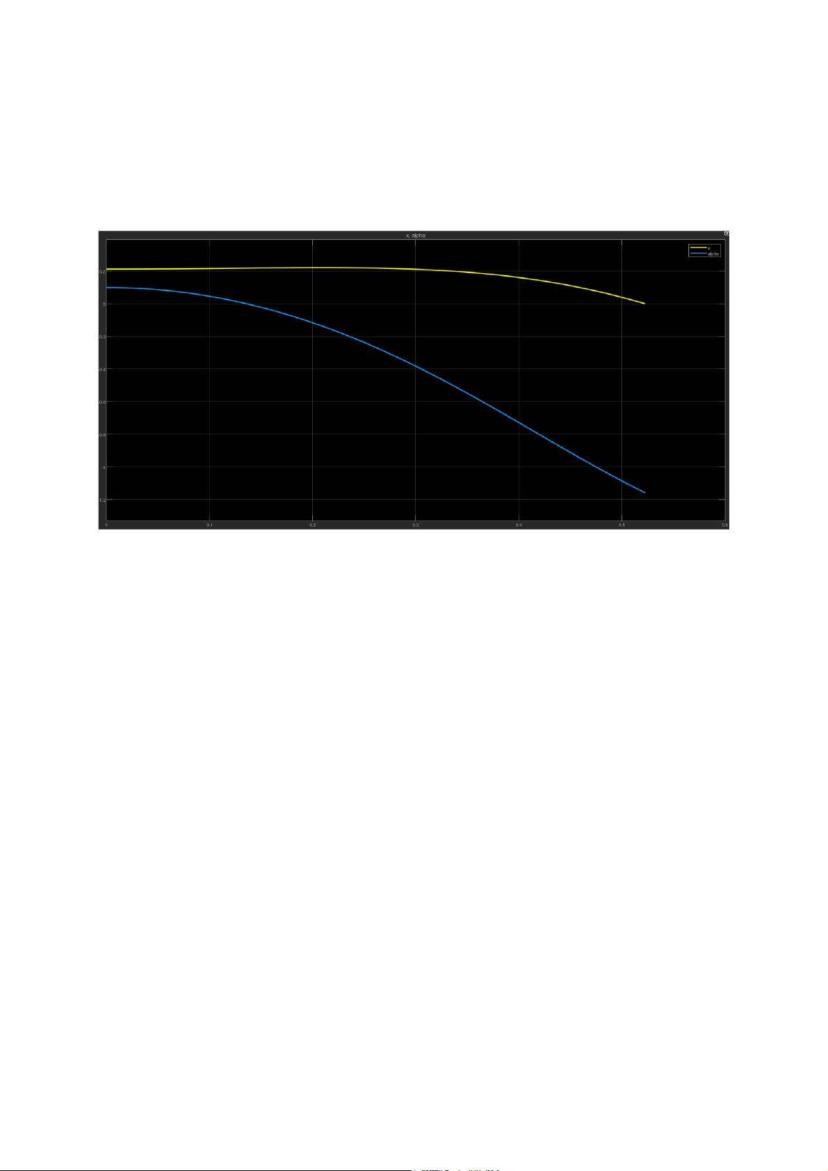
α= 0.1rad and x =L/2 to drop the ball at the midpoint of the beam. To ensure a more critical assessment
of our system, we set some boundaries to our model to stop the simulation if the ball should fall off
the beam (i.e., x<0 or x>L). The behaviour we observe in Figure 2 shows one we would expect. The
uncontrolled system has no ability to correct itself and so the ball falls off and the beam comes to rest
at an angle of ~90°.
Figure 2 Behaviour of uncontrolled Nonlinear system
System Analysis
It is vital that when modelling a system, the engineer understands the poles and zeros present, as well
as the controllability and observability of the system. For a continuous time model, we can assume
that any pole with a positive real part can be regarded as terminal and will ensure the system goes
unstable. The system initialised below shows the Linearised state space model.
A = [0 1 0 0; 0.0290 0 7.0062 0; 0 0 0 1; -3.1991 0 0.1088 0];
B = [0; -4.332; 0; 47.7514];
C = [1 0 0 0; 0 0 1 0];
D = [0];
sys = ss(A, B, C, D)
The poles and zeros of the system can be mapped in MATLAB by using the pzmap function.
[p, z] = pzmap(sys)
It is conclusive that there are 4 poles in the system lying at:
From this analysis we can see two poles with positive real parts, shown here as pole number 3 and 4.
It is critical that if the system is to be stable, these 2 poles must be brought back into the negative
plane.
Jack Gibson, Andreas Wiedholz, Jonathan Ott
Before designing the controller, it is also critical to determine if the system is controllable and/or
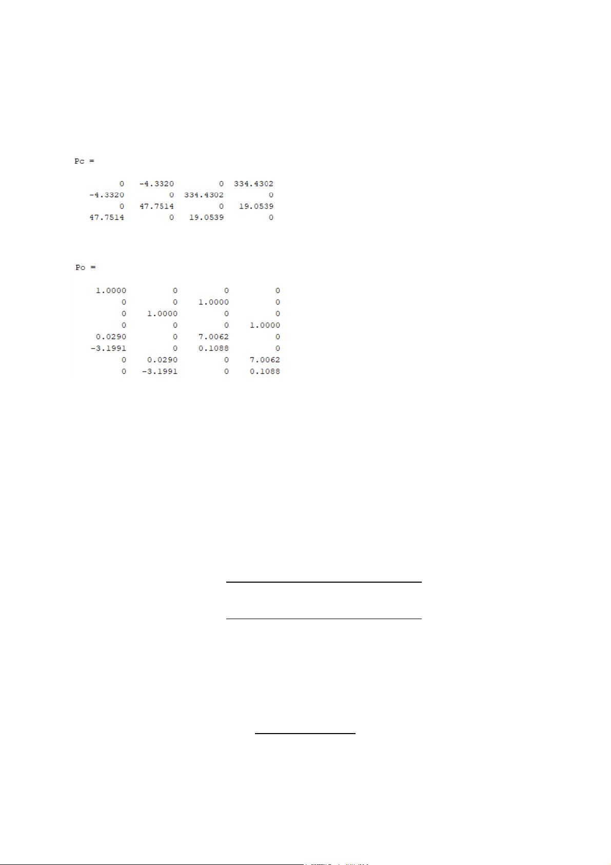
observable. In order to obtain these results two matrices, Pc and Po must be created,
Pc = [B A*B A*A*B A*A*A*B];
Po = [C; C*A; C*A*A; C*A*A*A];
We can conclude therefore that this system is both fully observable and controllable, as the rank of
these matrices can be determined as 4. If any other rank is detected we must conclude that the system
is uncontrollable and/or unobservable.
PID Controller
In this task a PID approach must be taken to control the system. The state space model can be
converted into two transfer functions to use the PID controller. This is done simply in MATLAB with
the command tf(sys).
As the ball beam system has two outputs to be controlled the result of this function is two transfer
functions, one for displacement ) and another for angular rotation of the beam. These transfer
functions are shown below:
The most trivial and highly effective method for tuning the PID controller is to use MATLAB’s SISO tool.
The transfer function is first loaded into the architecture of the closed loop feedback system and the
values of the PID can be manipulated to shift the poles to the desired location to achieve an acceptable
response.
The step response of this PID in the closed loop system looks like:


