没有合适的资源?快使用搜索试试~ 我知道了~
资源推荐
资源详情
资源评论


Team # 2202120
Problem Chosen
C
2022
MCM/ICM
Summary Sheet
Team Control Number
2202120
Data mining based quantitative trading strategy model for gold
and bitcoin
Summary
First, we first performed data cleaning on the data at hand. We first solved the
inconsistent format of Date column programmatically and sorted it, then we determined the
error value of value by box plot test and changed the error value to null value. Then the
vacant values and error values were filled using Newton interpolation based on time series.
The approximate trend of gold and bitcoin prices from September 11, 2016 onwards is
depicted by plotting a line graph.
For the first question, considering that the csv file only gives the relationship between
time and price, we used a time series ARIMA model to predict the price trend of gold and
bitcoin. First, we performed a smoothness test to find that the time series is unstable, then we
did a 1st order difference and the data passed the stability test. To avoid errors caused by
human subjectivity, we then plotted ACF and PACF charts, then determined the order of
the ARMA model for the two types of investment products by using the BIC information
criterion and the AIC information criterion, and fitted the model to predict the price for the
days after the closing to obtain the daily return after the closing, so as to build a dynamic
programming model to calculate the most optimal portfolio of positions.
For the second question, we use gradient descent to tune the parameters of the ARIMA
model to improve the model and obtain the optimal solution, thus obtaining the optimal
model. Then we give a perturbation to the trading strategy to see if the total return will
increase, and finally we confirm that this "seems" to be the optimal model.
For the third question, we were asked to perform a sensitivity test on the rate parameters.
We observed the final profitability results by increasing the two transaction costs rate
parameters
and
to 1-5 times and 1-3 times their original values, and obtained
that the data did not fluctuate much, indicating that the model has good stability.
For the sensitivity analysis, we also did other work. We changed the three parameters
, α and β of the ARIMA model in the first question separately, and compared the predicted
images after changing the parameters with the original images, and found that the change of
parameter β, i.e., the parameter of MA, had some sensitivity to the prediction results of
the model. And the model prediction results do not change much after the parameters
and β are changed.
Finally, we performed a model extension where we optimized the timing operation by
using several of the more established quantitative transaction timing theories in finance:
the Moving Average (MA) and KDJ indicators, and developed some trading rules for
existing products. The VaR risk control model is also used to assess the risk of the next
day's trading. When the possibility of losing money is assessed to be higher than 70%, an
early warning is made and the quantitative transaction process is suspended, allowing
the user to make his own choice and proceed to the next operation.
Keywords: Time Series Model Gradient descent method Sensitivity testing Quantitative
transaction Timing Theory VaR model

Team # 2202120 Page 1 of 23
Content
1. Introduction....................................................................................................................2
1.1 Problem Background…............................................................................................2
1.2 Restatement of the Problems....................................................................................2
1.3 Literature Review…………….................................................................................3
1.4 Our Work.................................................................................................................2
2. Assumptions and Justifications......................................................................................4
3. Notations Description....................................................................................................5
4. Establishment and Result of the Model.........................................................................6
4.1 Task One..................................................................................................................6
4.1.1 Model Preparations and Data Preprocessing ..................................................6
4.1.2 Analysis of the Problem...................................................................................8
4.1.3 Model Establishment........................................................................................8
4.1.4 Algorithm Design ...........................................................................................11
4.1.5 Solving the Problem........................................................................................12
4.2 Task Two................................................................................................................13
4.2.1 Model Preparations and Data Preprocessing ................................................13
4.2.2 Analysis of the Problem.................................................................................13
4.2.3 Improvement of Task One’s Model...............................................................13
4.2.4 Algorithm Design ..........................................................................................13
4.2.5 Solving the Problem.......................................................................................14
5. Sensitive Analysis and Task Three................................................................................14
5.1 Overview of sensitivity analysis.............................................................................14
5.2. Sensitivity analysis of dynamic planning models to rate parameters....................15
5.3 Sensitivity analysis of the three parameters of the ARMIA model........................15
6. Model Expansion...........................................................................................................16
6.1 Quantitative transaction Timing Theory Approach................................................16
6.1.1 Moving Average(MA) .............................................................................16
6.1.2 KDJ Indicators................................................................................................17
6.2 VaR Risk Control Model........................................................................................18
7. Strength and Weakness .................................................................................................19
7.1 The Strength of the model.......................................................................................19
7.2. The Weakness of the model...................................................................................19
8. Conclusion.....................................................................................................................20
MEMO...............................................................................................................................21
References..........................................................................................................................22
Programs............................................................................................................................23

Team # 2202120 Page 2 of 23
1. Introduction
1.1 Problem Background
Quantitative transaction was created after the 1950s and has been developed for nearly
70 years. It has developed more maturely around the world and has gradually become popular
in the capitalist markets of major countries[1].
Quantitative transaction refers to the use of computers to build mathematical models to
judge the timing of trading for buy and sell operations. While traditional securities trading
often relies on the subjectivity of traders, quantitative trading quantifies investment ideas[2]
and helps investors make objective and calm analysis and judgments by establishing
quantitative models with computers, reducing investment mistakes caused by investors'
impulsiveness and subjective judgments.
1.2 Restatement of the Problems
The first question of this problem asks to develop a Quantitative transaction strategy
model with the gold and bitcoin trading data in our hand and calculate the profit outcome of
an initial $1,000 investment on September 10, 2021.
The second question asks us to argue that the model provides the best strategy.
The third question asks us to perform a sensitivity analysis to indicate the impact that
transaction costs have on the quantitative trading strategy and results we have developed.
The final question is asking us to write a two-page memo including the strategy, model,
and results to our investors.
1.3 Literature Review
This problem requires us to develop a model that provides the best trading strategy.
Such a model is known as a quantitative trading model in the field of finance and is one of
the hot research topics in finance today[3].
Most of the domestic and international research hotspots on quantitative trading are on
how to predict the stock or futures movements on this point[4], and scholars mostly use
Probit models for data mining, and machine learning models such as Bayesian networks and
support vector machines, and not a few use deep learning models such as artificial neural
networks. Most of them have huge amount of data and labels[5], however, this competition
limited the data parameters to only two labels, time and price. Obviously, it is not feasible to
apply common models and algorithms here.

Team # 2202120 Page 3 of 23
1.4 Our Work
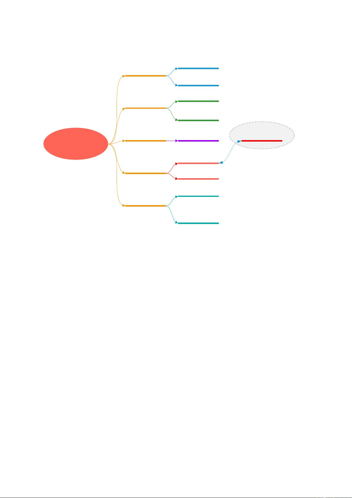
Figure 1. Summary of Our Work
First, we first did a general overview of the data at hand and found that there were errors
and missing data, so we performed a data cleaning exercise. We uniformly formatted the
dates in the csv files by writing Python code, then used box plots test to determine the error
values of the values and changed the checked error values to null values. Then, we fill the
vacant and error values using Newton interpolation based on time series. Finally, by
plotting the line graphs of the trend of gold and bitcoin prices from September 11, 2016, and
comparing the line graphs in the title overview, we found roughly the same, which shows that
our data cleaning efforts were successful.
In the second step, we proceeded to solve the first half of the first question, which is to
predict the price after a certain day from the original price time series and thus calculate the
return of the latter days. After thinking about it, we found that only time and price were given
in the table, so we used the time series model ARIMA, we performed the usual smoothness
test and found that the time series was unstable, so we did a first order difference operation
to get the new time series, and then performed the smoothness test we found that the new
series was roughly smooth. Then, our team plotted ACF and PACF plots to determine the
approximate order range of p and q parameters, and then determined the order of ARMA
models for both types of investment products by using the BIC information criterion and
AIC information criterion, both of which are ARMA (1, 1, 1). Finally, the model is fitted to
Our Work
Data Cleaning
Task One
Task Two
Sensitive Analysis
Model Expansion
Gradient Descent
VaR Model
Quantitative
Transaction Timing
Theories
Sensitive Analysis of
ARIMA s Parameters
Task Three
Dynamic
Programming
ARIMA
Box Plots Test
Newton Interpolation
Based on Timeseries
Sensitive Analysis of
Transaction Costs

Team # 2202120 Page 4 of 23
predict the price for the days after the closing, which is used to calculate the return for each
day after the closing, so that a dynamic programming model can be built to calculate the
optimal portfolio of positions. We use Python's SciPy library to solve the dynamic
programming model and finally obtain the optimal solution for the ratio of gold and bitcoin
positions in the short term.
In the third step, we argue for the optimality of the model as required. In fact, the
ARIMA model has inherent shortcomings, which we list in Section 7. Second, the data in the
table contain only time and price, and it is also not reasonable to infer prices from time alone.
In summary, the model we obtained in the first question is only the optimal solution by
dynamic programming model on the prediction result of ARIMA model, it cannot be optimal
globally, so we tried to find the "optimal strategy" by adjusting the parameters of the original
model by gradient descent method, and after testing we proved that our model seems to be
After testing, we proved that our model seems to be "optimal".
In the fourth step, we performed sensitivity analysis on the gold and bitcoin trading rate
parameters as required. We observed the final profitability results by increasing the two rate
parameters
and
to 1-5 times and 1-3 times of the original, and obtained little
data fluctuation, indicating that the model has good stability.
For the sensitivity analysis, we also did other work. We changed the three parameters
, α and β of the ARIMA model in the first question separately, and compared the predicted
images after changing the parameters with the original images, and found that the change of
parameter β, i.e., the parameter of MA, had some sensitivity to the prediction results of
the model. And the model prediction results do not change much after the parameters
and β are changed.
Finally, we have improved our model in the model extension section. We optimized our
trading timing operations by using several of the more established quantitative transaction
timing theories in finance: moving averages (MA) and KDJ indicators[6], and developed
some trading rules for existing products that have a higher priority than the ARIMA model
prediction results. We tested our program and the results showed a large degree of
improvement in our model.
At the same time, we use the VaR risk control model[7] to assess the risk of the next
day's trading. When the possibility of losing money is assessed to be higher than 70%, we
make an early warning and suspend the quantitative trading program, allowing the
user to choose, and proceed to the next operation.
2. Assumptions and Justifications
⚫ Assumption1: The data given in the table are all true and reliable.
剩余23页未读,继续阅读
TIM33470348
- 粉丝: 4591
- 资源: 3

上传资源 快速赚钱
我的内容管理 收起
我的资源 快来上传第一个资源
我的收益
登录查看自己的收益我的积分 登录查看自己的积分
我的C币 登录后查看C币余额
我的收藏
我的下载
下载帮助

会员权益专享
安全验证
文档复制为VIP权益,开通VIP直接复制

- 1
- 2
- 3
- 4
- 5
- 6
前往页