


Functions and Models
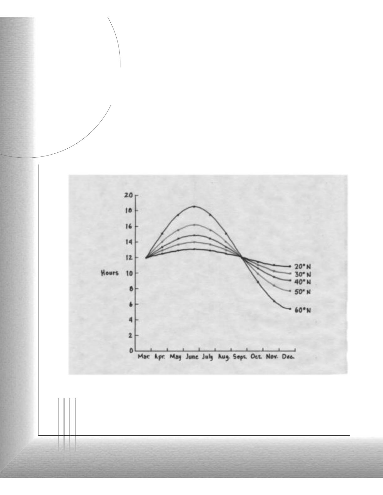
A graphical representation of a function––here the
number of hours of daylight as a function of the time
of year at various latitudes–– is often the most nat-
ural and convenient way to represent the function.
The fundamental objects that we deal with in calculus are
functions. This chapter prepares the way for calculus by
discussing the basic ideas concerning functions, their
graphs, and ways of transforming and combining them.
We stress that a function can be represented in different
ways: by an equation, in a table, by a graph, or in words. We look at the main
types of functions that occur in calculus and describe the process of using these func-
tions as mathematical models of real-world phenomena. We also discuss the use of
graphing calculators and graphing software for computers.
||||
1.1 Four Ways to Represent a Function
Functions arise whenever one quantity depends on another. Consider the following four
situations.
A. The area of a circle depends on the radius of the circle. The rule that connects
and is given by the equation . With each positive number there is associ-
ated one value of , and we say that is a function of .
B. The human population of the world depends on the time . The table gives estimates
of the world population at time for certain years. For instance,
But for each value of the time there is a corresponding value of and we say that
is a function of .
C. The cost of mailing a first-class letter depends on the weight of the letter.
Although there is no simple formula that connects and , the post office has a rule
for determining when is known.
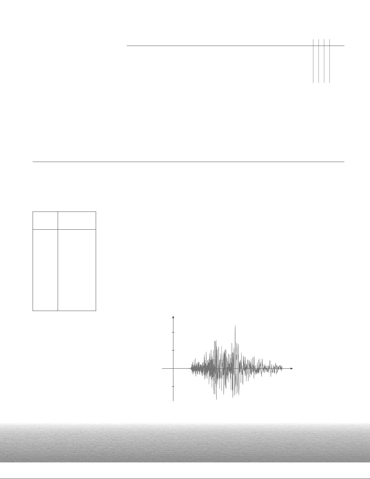
D. The vertical acceleration of the ground as measured by a seismograph during an
earthquake is a function of the elapsed time Figure 1 shows a graph generated by
seismic activity during the Northridge earthquake that shook Los Angeles in 1994.
For a given value of the graph provides a corresponding value of .
FIGURE 1
Vertical ground acceleration during
the Northridge earthquake
{cm/s@}
(seconds)
Calif. Dept. of Mines and Geology
5
50
10 15 20 25
a
t
100
30
_50
at,
t.
a
wC
Cw
w
C
tP
P,t
P19502,560,000,000
t,Pt
tP
rAA
rA
r
2
A
rrA
Population
Year (millions)
1900 1650
1910 1750
1920 1860
1930 2070
1940 2300
1950 2560
1960 3040
1970 3710
1980 4450
1990 5280
2000 6080
Each of these examples describes a rule whereby, given a number ( , , , or ), another
number ( , , , or ) is assigned. In each case we say that the second number is a func-
tion of the first number.
A function is a rule that assigns to each element in a set exactly one ele-
ment, called , in a set .
We usually consider functions for which the sets and are sets of real numbers. The
set is called the domain of the function. The number is the value of at and is
read “ of .” The range of is the set of all possible values of as varies through-
out the domain. A symbol that represents an arbitrary number in the domain of a function
is called an independent variable. A symbol that represents a number in the range of
is called a dependent variable. In Example A, for instance, r is the independent variable
and A is the dependent variable.
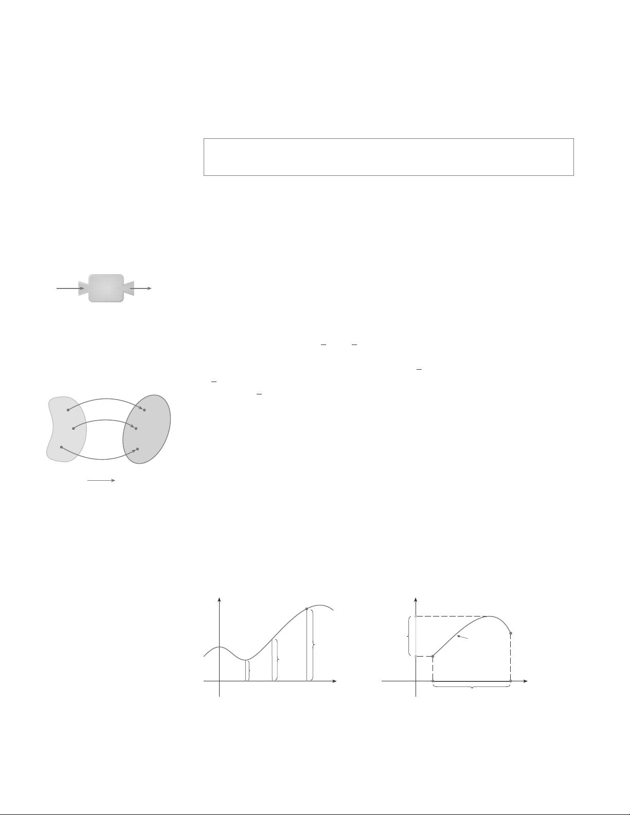
It’s helpful to think of a function as a machine (see Figure 2). If is in the domain of
the function then when enters the machine, it’s accepted as an input and the machine
produces an output according to the rule of the function. Thus, we can think of the
domain as the set of all possible inputs and the range as the set of all possible outputs.
The preprogrammed functions in a calculator are good examples of a function as a
machine. For example, the square root key on your calculator computes such a function.
You press the key labeled
(
or
)
and enter the input x
. If , then is not in the
domain of this function; that is, is not an acceptable input, and the calculator will indi-
cate an error. If , then an approximation to will appear in the display. Thus, the
key on your calculator is not quite the same as the exact mathematical function defined
by .
Another way to picture a function is by an arrow diagram as in Figure 3. Each arrow
connects an element of to an element of . The arrow indicates that is associated
with is associated with , and so on.
The most common method for visualizing a function is its graph. If is a function with
domain , then its graph is the set of ordered pairs
(Notice that these are input-output pairs.) In other words, the graph of consists of all
points in the coordinate plane such that and is in the domain of .
The graph of a function gives us a useful picture of the behavior or “life history” of
a function. Since the -coordinate of any point on the graph is , we can read
the value of from the graph as being the height of the graph above the point (see
Figure 4). The graph of also allows us to picture the domain of on the -axis and its
range on the -axis as in Figure 5.
0
x
y ƒ(x)
domain
range
y
FIGURE 4
{
x, ƒ
}
ƒ
f(1)
f(2)
x
y
0
12 x
FIGURE 5
y
xff
xf x
y f xx, yy
f
fxy f xx, y
f
x, f x
x A
A
f
af ax,
f xBA
f x
s
x
f
s
x
s
xx 0
x
xx
0
s
x
s
f x
xf,
x
ff
xf xfxf
xffxA
BA
Bf x
Axf
aCPA
twtr
12
❙❙❙❙
CHAPTER 1 FUNCTIONS AND MODELS
FIGURE 2
Machine diagram for a function ƒ
x
(input)
ƒ
(output)
f
f
A
B
ƒ
f(a)
a
x
FIGURE 3
Arrow diagram for ƒ

SECTION 1.1 FOUR WAYS TO REPRESENT A FUNCTION
❙❙❙❙
13
EXAMPLE 1 The graph of a function is shown in Figure 6.
(a) Find the values of and .
(b) What are the domain and range of ?
SOLUTION
(a) We see from Figure 6 that the point lies on the graph of , so the value of at
1 is . (In other words, the point on the graph that lies above x 1 is 3 units
above the x-axis.)
When x 5, the graph lies about 0.7 unit below the x-axis, so we estimate that
.
(b) We see that is defined when , so the domain of is the closed inter-
val . Notice that takes on all values from 2 to 4, so the range of is
EXAMPLE 2 Sketch the graph and find the domain and range of each function.
(a) (b)
SOLUTION
(a) The equation of the graph is , and we recognize this as being the equa-
tion of a line with slope 2 and y-intercept 1. (Recall the slope-intercept form of the
equation of a line: . See Appendix B.) This enables us to sketch the graph of
in Figure 7. The expression is defined for all real numbers, so the domain of
is the set of all real numbers, which we denote by . The graph shows that the range is
also .
(b) Since and , we could plot the points and
, together with a few other points on the graph, and join them to produce the
graph (Figure 8). The equation of the graph is , which represents a parabola (see
Appendix C). The domain of t is . The range of t consists of all values of , that is,
all numbers of the form . But for all numbers x and any positive number y is a
square. So the range of t is . This can also be seen from Figure 8.
(_1,1)
(2,4)
0
y
1
x
1
y=≈
FIGURE 8
y
y 0 0,
x
2
0x
2
tx
y x
2
1, 1
2, 4t1 1
2
1t2 2
2
4
f2x 1f
y mx b
y 2x 1
tx x
2
fx 2x 1
y
2 y 4 2, 4
ff0, 7
f0 x 7f x
f 50.7
f 1 3
ff1, 3
FIGURE 6
x
y
0
1
1
f
f 5f 1
f
|||| The notation for intervals is given in
Appendix A.
FIGURE 7
x
y=2x-1
0
-1
1
2
y
14
❙❙❙❙
CHAPTER 1 FUNCTIONS AND MODELS
Representations of Functions
There are four possible ways to represent a function:
■■
verbally (by a description in words)
■■
numerically (by a table of values)
■■
visually (by a graph)
■■
algebraically (by an explicit formula)
If a single function can be represented in all four ways, it is often useful to go from one
representation to another to gain additional insight into the function. (In Example 2, for
instance, we started with algebraic formulas and then obtained the graphs.) But certain
functions are described more naturally by one method than by another. With this in mind,
let’s reexamine the four situations that we considered at the beginning of this section.
A. The most useful representation of the area of a circle as a function of its radius is
probably the algebraic formula , though it is possible to compile a table of
values or to sketch a graph (half a parabola). Because a circle has to have a positive
radius, the domain is , and the range is also .
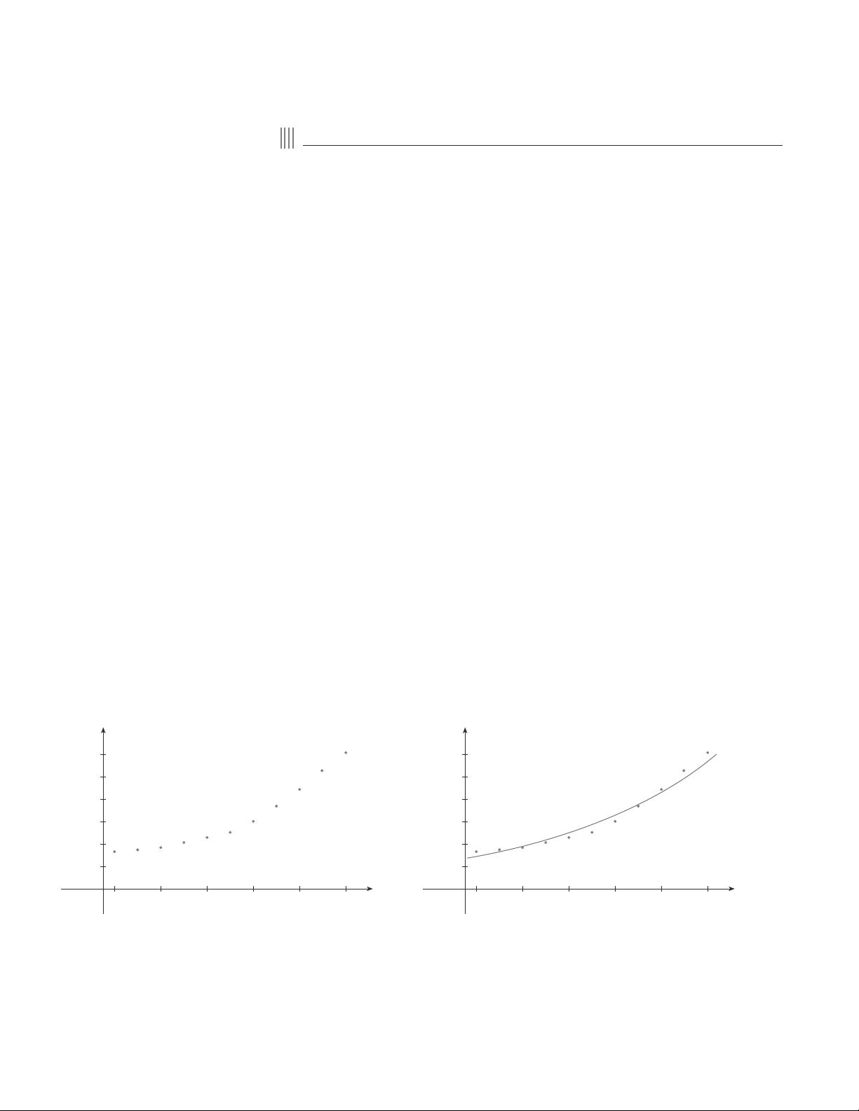
B. We are given a description of the function in words: is the human population of
the world at time t. The table of values of world population on page 11 provides a
convenient representation of this function. If we plot these values, we get the graph
(called a scatter plot) in Figure 9. It too is a useful representation; the graph allows us
to absorb all the data at once. What about a formula? Of course, it’s impossible to
devise an explicit formula that gives the exact human population at any time t.
But it is possible to find an expression for a function that approximates . In fact,
using methods explained in Section 1.5, we obtain the approximation
and Figure 10 shows that it is a reasonably good “fit.” The function is called a
mathematical model for population growth. In other words, it is a function with an
explicit formula that approximates the behavior of our given function. We will see,
however, that the ideas of calculus can be applied to a table of values; an explicit
formula is not necessary.
FIGURE 10FIGURE 9
1900
6x10'
P
t
1920 1940 1960 1980 2000 1900
6x10'
P
t
1920 1940 1960 1980 2000
f
Ptf t 0.008079266 1.013731
t
Pt
Pt
Pt
0, r
r 0 0,
Ar
r
2


