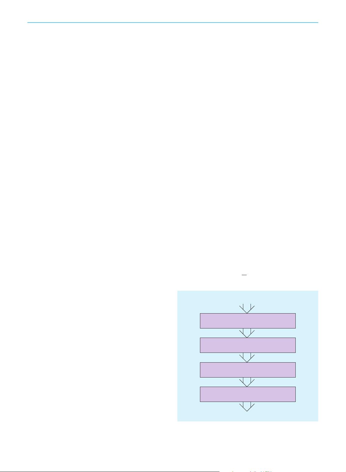
steps 1 and 2 or steps 1–3 in one shot; see the “Differential
Constraints” section. The eventual need for feedback in Step 4
motivates the direct computation of a feedback plan, which is
covered in the “Feedback Motion Planning” section.
Another issue with the framework in Figure 1, which is
perhaps more subtle, is that this fixed decomposition of the
overall problem of getting a robot to navigate has artificially
inflated the information requirements. The framework
requires that powerful sensors, combined with strong prior
knowledge, must be providing accurate state estimates at all
times, including the robot configuration, velocity components,
and obstacle models. This unfortunately overlooks a tremen-
dous opportunity to reduce the overall system complexity by
sensing just enough information to complete the task. In this
case, a plan is p : I!U instead of p : X ! U,inwhichI
is a specific information space that can be derived from sensor
measurements and from which a complete reconstruction of
the state x(t) 2 X is either impossible or undesirable. The
“Sensing Uncertainty” section introduces sensing, filtering,
and planning from this perspective: The state cannot be fully
estimated, but tasks are nevertheless achieved.
Differential Constraints
In this section, it may help to imagine that the C-space C is
R
n
to avoid the manifold technicalities from Part I. In the
models and methods of Part I, it was assumed that a path
can be easily determined between any two configurations
in the absence of obstacles. For example, vertices in the
trapezoidal decomposition approach are connected by a
straight line segment in the collision-free region, C
free
. This
section complicates the problem by introducing differen-
tial constraints, which restrict the allowable velocities at
each point in C
free
. These are local constraints in contrast
to the global constraints that arise due to obstacles.
Differential constraints naturally arise from the kinemat-
ics and dynamics of robots. Rather than treating them as an
afterthought, this section discusses how to directly model
and incorporate them into the planning process. In this
way, a path is produced that already satisfies the constraints.
Modeling the Constraints
For simplicity, suppose C¼R
2
.Let
_
q ¼ (
_
x,
_
y)denotea
velocity vector in which
_
x ¼ dx=dt and
_
y ¼ dy=dt.Starting
from any point in R
2
, say (0, 0), consi der what paths can
possibly be produced by integrating the velocity:
~
q(t) ¼
R
t
0
_
q(s)ds. Here,
_
q is interpreted as a function of
time. If no constraints are imposed on
_
q (other than require-
ments for integrability), then the trajectory
~
q is virtually
unrestricted. If, however, we require
_
x > 0, then the only
trajectories for which x monotonically increases are allowed.
If we further constrain it so that 0 <
_
x 1, then the rate at
which x increases is bounded. If time was measured in sec-
onds and R
2
in meters, then
~
q must cause travel in the x
direction with a rate of no more than 1 m/s.
More generally, we want to express a set of allowable
velocity vectors
_
q ¼ (
_
x,
_
y) for every q ¼ (x, y) 2 R
2
. Rather
than write a set-valued function with domain R
2
, a more
compact, convenient method is to define a function f that
yields
_
q as a function of q and a new parameter u:
_
q ¼ f (q, u): (1)
This results in a velocity-valued function called the
configuration-transition equation, which indicates the
required velocity vector, given q and u. The parameter u is
called an action (or input) and is chosen from a predeter-
mined action space U.Sincef is a function of two variables,
there are two convenient interpretations by holding each
variable fixed: 1) if q is held fixed, then each u 2 U produces
a possible velocity
_
q at q; in other words, u parameterizes
the set of possible velocities; 2) if u is fixed, then f specifies a
velocity at every q; this results in a vector field over C.
For a common example of the configuration-transition
equation, Figure 2 shows a carlike robot that has the C-
space of a rigid body in the plane: C¼R
2
3 S
1
. The config-
uration vector is q ¼ (x, y, h). Imagine that the car drives
around slowly (so that dynamics are ignored) in an infinite
parking lot. Let / be the steering angle of the front tires, as
shown in Figure 2. If driven forward, the car will roll along
a circle of radius q. Note that it is impossible to move the
center of the rear axle laterally because the rear wheels
would skid instead of roll. This induces the constraint
_
y=
_
x ¼ tan h. This constraint, along with another due to the
steering angle, can be converted into the following form
(see [12, section 13.1.2.1]):
_
x ¼ u
s
cos h
_
y ¼ u
s
sin h
_
h ¼
u
s
L
tan u
/
, (2)
Compute a Collision-Free Path
t : [0, 1] S C
free
Smooth t to Satisfy Differential Constraints
σ : [0, 1] S C
free
Execute π on the Robot
Complete Geometric Model of the World
Step 1
Step 2
Step 3
Step 4
Design a Trajectory That Follows σ
q : [0, t ] S C
free
~
Design a Feedback Controller to Track q
π : X S U
~
Figure 1. The long road to using a computed collision-free path.
Note that complete, perfect knowledge of the robot and obstacles
enters in, and sensors are utilized only during the final execution.
JUNE 2011
•
IEEE ROBOTICS & AUTOMATION MAGAZINE
•
109
•


 我的内容管理
展开
 我的资源
快来上传第一个资源
 我的收益 登录查看自己的收益
 我的积分
登录查看自己的积分
 我的C币
登录后查看C币余额
 我的收藏
我的收藏  我的下载
我的下载  下载帮助
下载帮助 
 前往需求广场,查看用户热搜

 信息提交成功