没有合适的资源?快使用搜索试试~ 我知道了~
资源详情
资源评论
资源推荐
Dynamical Models in Biology
* Publisher: Academic Press
* Number of Pages: 187
* Publication Date: 2001-05-23
* Sales Rank: 2014036
* ISBN / ASIN: 0122491033
* EAN: 9780122491030
* Binding: Hardcover
* Manufacturer: Academic Press
* Studio: Academic Press
* Copyright 2001 Elsevier Inc. All rights reserved
* Author(s): Miklos Fakars
Table of Contents
Chapter 1 - Discrete population models, 1-15
Chapter 2 - Population dynamics in continuous time, 17-61
Chapter 3 - Epidemics, 63-77
Chapter 4 - Evolution and population genetics, 79-104
Chapter 5 - Morphogenesis and pattern formation, 105-123
Appendix 1 - Discrete mathematics, 125-141
Appendix 2 - Ordinary differential equations, 143-156
Appendix 3 - Partial differential equations, 157-169
Appendix 4 - Riemannian geometry, 171-177
References, 179-183
Index, 184-187
Chapter 1
DISCRETE POPULATION
MODELS
Population dynamics looks at the problem of how the number, the quantity of
a well-defined group of living creatures, a species or a system of species, that is,
those that share a common habitat, varies in time. Living creatures are born,
reproduce, and die at a certain rate that depends on circumstances, including
their specific genetically determined properties, the quantity of food available,
their own density etc., and in case of a shared habitat, on the properties of
those species with whom they live together. In this chapter we deal first with
species of nonoverlappmg generations. This means that the parent generation
has disappeared by the time the next generation is born. One may imagine
some insects that lay their eggs in the soil in the autumn and then die while the
next generation is born the next spring. Next we consider a single species with
discrete age groups.
1.1 Nonoverlapping Generations and Discrete
Time Models
In this Section a single isolated population will be considered first. Its number
or abundance at time t is denoted by Nt- Time is measured in discrete units
(seconds, hours, years etc.) and it is assumed that the number of the genera-
tion of the moment (year etc.) t determines the number of the next generation,
that is, the number Nt+i- In other words, this means that the previous gen-
erations infiuence the abundance of the generation at time t + 1 only through
the generation at time t. It is also assumed that the circumstances that may
have an effect on reproduction, food, temperature etc. remain the same, for
example, each year is like the previous one. Consider the difference between the
numbers of the (t + l)st and the tth generation. If we divide this difference by
the quantity of the tth generation we obtain the per capita growth rate at time
2 Discrete Population Models
t.
It
is usually given in percentages. Population dynamics depends on how this
per capita growth rate
at
time
t
depends on the actual size of the population.
The simplest assumption is that this rate is constant. If this constant is nega-
tive then this means that there are fewer in each successive generation. If this
negative rate is constant, the obvious consequence is
a
population that dies out
rapidly. If this constant is positive then the equation that governs the dynamics
[Nt+i
-
Nt)
/Nt = r,
where the constant
r > 0
is now the per capita growth rate of the population.
This equation can be written in the form
Nt+i
=
{I + r) Nt
.
(1.1.1)
If we express the number at time
t
+ 2 by the number at time
t
+ 1, and then the
number
at
time
t +
3 by the number
at
time
t
+ 2 and so on, then the number
of the generation
at
time
t
+
n
will be
Nt+n
=
(1
+ rf
Nt
.
As
r >
0, this clearly means that the numbers go to infinity as time increases in-
definitely. If the per capita growth rate is, for example, 2%, then the hundredth
generation numbers
1.02^'^'^
=
7.24 times as much as the original one. In Nature
such exponential growth cannot go on indefinitely because some limiting factor
of the environment, lack of food, oxygen, space etc. or simply the adverse effects
of overcrowding, slows down growth sooner or later. We arrive at
a
more realis-
tic model if we assume that the per capita growth rate is
a
decreasing function
of the abundance of the population, which equals zero when the size of the pop-
ulation reaches the maximum that can be maintained by the environment. The
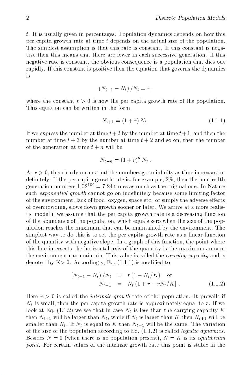
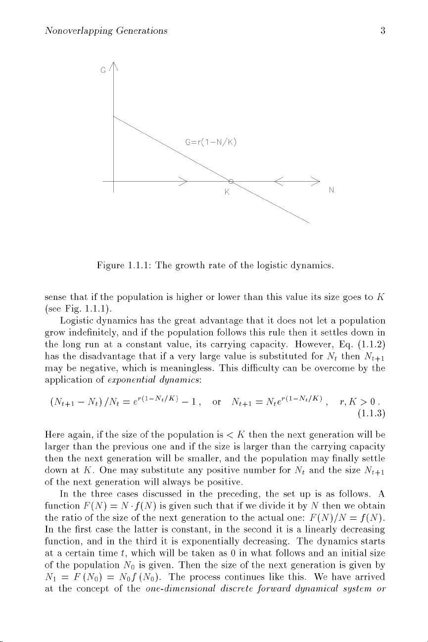
simplest way to do this is to set the per capita growth rate as
a
linear function
of the quantity with negative slope. In
a
graph of this function, the point where
this line intersects the horizontal axis of the quantity is the maximum amount
the environment can maintain. This value is called the carrying capacity and is
denoted by K> 0. Accordingly, Eq. (1.1.1) is modified to
[Nt+i-Nt)/Nt = r{l-Nt/K) or
Nt+i = Ntil
+
r-rNt/K] .
(1.1.2)
Here
r > 0 is
called the intrinsic growth rate of the population.
It
prevails if
Nt is small; then the per capita growth rate is approximately equal to
r.
If we
look
at
Eq. (1.1.2) we see that in case
Nt
is less than the carrying capacity
K
then Nt+i will be larger than Nt, while if Nt is larger than
K
then Nt+i will be
smaller than Nt- If Nt is equal to
K
then Nt+i will be the same. The variation
of the size of the population according to Eq. (1.1.2) is called logistic dynamics.
Besides
N
= 0 (when there is no population present),
N = K
is its equilibrium
point. For certain values of the intrinsic growth rate this point is stable in the
Nonoverlapping Generations
Figure 1.1.1: The growth rate of the logistic dynamics.
sense that if the population is higher or lower than this value its size goes to K
(see Fig.
1.1.1).
Logistic dynamics has the great advantage that it does not let a population
grow indefinitely, and if the population follows this rule then it settles down in
the long run at a constant value, its carrying capacity. However, Eq. (1.1.2)
has the disadvantage that if a very large value is substituted for Nt then Nt+i
may be negative, which is meaningless. This difficulty can be overcome by the
application of exponential dynamics:
{Nt+,
- Nt) /Nt =
e'-(i-^'/^)
1
N
t+i
jy gril-m/K)
r. A' > 0 .
(1.1.3)
Here again, if the size of the population is < K then the next generation will be
larger than the previous one and if the size is larger than the carrying capacity
then the next generation will be smaller, and the population may finally settle
down at K. One may substitute any positive number for Nt and the size Nt+i
of the next generation will always be positive.
In the three cases discussed in the preceding, the set up is as follows. A
function F{N) = N
•
f{N) is given such that if we divide it by N then we obtain
the ratio of the size of the next generation to the actual one: F{N)/N = f{N).
In the first case the latter is constant, in the second it is a linearly decreasing
function, and in the third it is exponentially decreasing. The dynamics starts
at a certain time t, which will be taken as 0 in what follows and an initial size
of the population NQ is given. Then the size of the next generation is given by
Ni = F (No) = Nof (No). The process continues like this. We have arrived
at the concept of the one-dimensional discrete forward dynamical system or
剩余181页未读,继续阅读
gongchang02
- 粉丝: 2
- 资源: 47
上传资源 快速赚钱
- 我的内容管理 展开
- 我的资源 快来上传第一个资源
- 我的收益 登录查看自己的收益
- 我的积分 登录查看自己的积分
- 我的C币 登录后查看C币余额
- 我的收藏
- 我的下载
- 下载帮助
最新资源
- 实现了7种排序算法.三种复杂度排序.三种nlogn复杂度排序(堆排序,归并排序,快速排序)一种线性复杂度的排序.zip
- 冒泡排序 直接选择排序 直接插入排序 随机快速排序 归并排序 堆排序.zip
- 课设-内部排序算法比较 包括冒泡排序、直接插入排序、简单选择排序、快速排序、希尔排序、归并排序和堆排序.zip
- Python排序算法.zip
- C语言实现直接插入排序、希尔排序、选择排序、冒泡排序、堆排序、快速排序、归并排序、计数排序,并带图详解.zip
- 常用工具集参考用于图像等数据处理
- 音乐展示网页、基于Stenography的图像数字水印添加与提取,以及基于颜色矩和Tamura算法的图像相似度评估算法py源码
- 基于EmguCV(OpenCV .net封装),图像数字水印加解密算法的实现,其中包含最低有效位算法,离散傅里叶变换算法+文档书
- 基于matlab+DWT的图像水印项目,数字水印+源代码+文档说明+图片+报告pdf
- (优秀毕业设计)基于python实现的数字图像可视化水印系统的设计与实现,多种数字算法实现+源代码+文档说明+理论演示pdf
资源上传下载、课程学习等过程中有任何疑问或建议,欢迎提出宝贵意见哦~我们会及时处理!
点击此处反馈
安全验证
文档复制为VIP权益,开通VIP直接复制
信息提交成功
评论9