


Artificial Neural Networks (ANN)
1 Introduction
Artificial neural networks are loosely based on the neural structure of the brain. The
human brain contains approximately 100 billion neurons. A typical neuron is
illustrated in simplified form in Figure 1.1.
Figure 1.1: Representation of Biological Neuron
1
In the human brain the neuron cell receives electrical input signals via a host of
dendrites. The cell effectively sums all the inputs from these dendrites and providing
the excitatory input is larger than the inhibitory input, and a defined threshold is
exceeded, a spike of energy is sent down the axon. The end of the axon splits into
thousands of branches which connect to the dendrites of adjacent neurons.
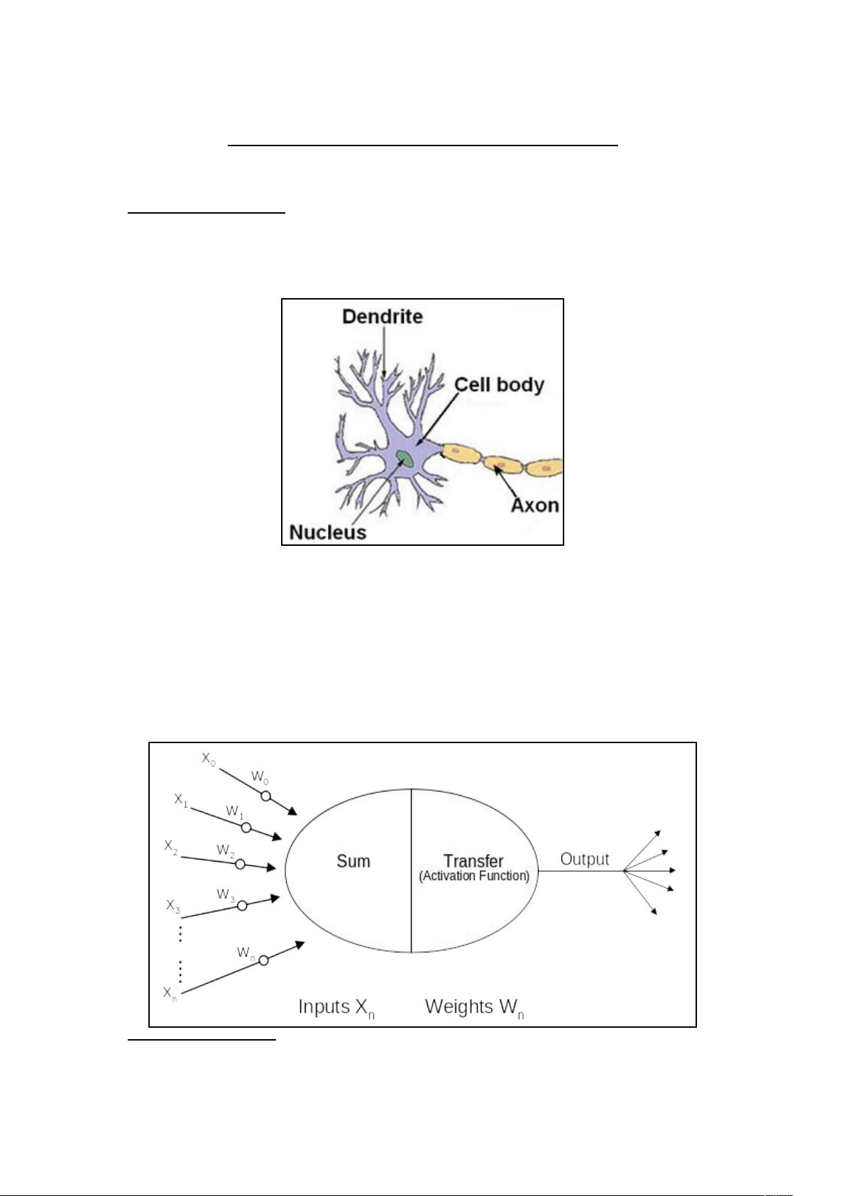
Artificial neurons attempt to simulate this operation as shown by Figure 1.2.
1
Wikipedia Foundation inc (2005) [Accessed October 2005]. Neuron. <http://en.wikipedia.org/
wiki/Neuron>
18/06/2022 Neural Network Notes Page 1 of 28
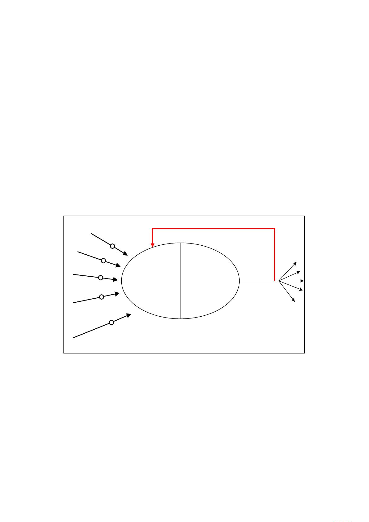
Figure 1.2: Representation of Artificial Neuron
2
The inputs into the neuron (shown as X
0
– X
n
) together with their connection weights
(W
0
– W
n
) represent the varying inhibitory and excitatory signals that travel down the
dendrites. Inside the neuron these inputs are summed and then a transfer function is
applied to produce a representative output, typically between 0 and 1 or -1 to +1.
Individual neurons may be connected, via their inputs and outputs, to a host of other
neurons in a variety of configurations to produce an artificial neural network.
In 1949 Donald Hebb
3
postulated the idea of Hebbian learning which states that
during learning the biological neurons synaptic connection strengths are adjusted to
increase efficiency along the selected neural pathway. This can be demonstrated by
conditioning where a subject can be taught to associate one event with another
unrelated event. For example Ivan Pavlov’s
4
conditioning experiments where dogs
learnt to associate the sound of a bell with the imminent arrival of food, thereby
stimulating the natural flow of saliva from the associated event (bell ringing).
Artificial neurons can simulate learning by providing a feedback mechanism to adjust
the individual input weights. This is illustrated in Figure 1.3.
Sum Transfer
(Activation Function)
W
0
W
1
W
2
W
3
W
n
Output
X
0
X
1
X
2
X
3
X
n
.
.
.
.
.
.
.
Inputs X
n
Weights W
n
Feedback to adjust Weights
Figure 1.3: Artificial Neuron with Feedback
By constantly updating the individual weights the network can be stabilised against a
particular problem domain. This forms the basis of the training, validation, and test
routines that are discussed later.
1.1 Artificial neural networks vs traditional computing
Traditional computing methods adhere to the Von Neumann architecture where
operations are carried out in a sequential well defined order. However, although
extremely quick at well defined problems (such as mathematical solutions, or
repetitive tasks), the Von Neumann model lacks the ability to generalise, associate or
predict to any degree of certainty. Tasks such as pattern recognition, and reasoning
18/06/2022 Neural Network Notes Page 2 of 28

with incomplete knowledge are better suited to an alternative approach. Artificial
neural networks offer this alternative approach. They provide the ability to learn from
the input data they are given and then apply this to unknown data, in effect they can
generalise and associate unknown data. Table 1.1 highlights these differences
Feature Von Neumann Neural Network
Processing Serial – Single Processor Parallel Processing
Fault Tolerant None Significant element
Programming Rule based Self programming
Learning None Continuously adaptable
Speed Quick at defined tasks Needs time to learn
Table 1.1: Comparison between Von Neumann and Neural Networks
5
1.2 Types of neural network
Although there are a multitude of neural network topologies there are 3 main
categories of network:
1. Back Propagation Networks
2. Recurrent Network
3. Self Organised Feature Maps
These networks can carry out a range of tasks such as data classification and decision
modelling, image and character recognition, pattern completion, and noise filtering
and reduction systems.
18/06/2022 Neural Network Notes Page 3 of 28

2 Back Propagation Networks
Back propagation feed forward networks are generally used for classification
purposes. The most common type is the Multilayer Perceptron (MLP). The MLP
consists of several layers of neurons, nominally an input layer, one or more hidden
layers, and an output layer. This is illustrated in Figures 2.1a and 2.1b.
Figure 2.1a: Single Output MLP Figure 2.1b: Multiple Outputs MLP
Classification generally falls into two areas:
i. Single output classification (Yes / No, on / off) – where the required output is
simply a two choice decision. The level of activation of the output neuron can
be used as an indication of the confidence of the decision.
ii. Multiple output classification – each output neuron is associated with a
particular class so for any given input only one output neuron will be
activated. For solutions with many classes it may be possible to use a binary
code output as illustrated in Table 2.1.
Output Neuron Activations (1 = On, 0 = Off)
Class Neuron A Neuron B Neuron C
A 0 0 0
B 0 0 1
C 0 1 0
D 0 1 1
E 1 0 0
F 1 0 1
G 1 1 0
H 1 1 1
Table 2.1: Using 3 output neurons to represent 8 classes
Before the network can begin classifying live data it must be trained to associate
particular input data with a particular class. It is important that a wide selection of
training data, representing each of the classes required, is used so that the network
will be more likely to correctly classify unknown data during live use.
18/06/2022 Neural Network Notes Page 4 of 28

2.1 Training
Training the MLP usually involves two distinct actions, a forward pass through the
network where an output is generated from a set of input data, and a backward pass
where any discrepancies between the actual output and the desired output are fed back
through the network to adjust individual weights and biases.
2.1.1 Feed forward cycle
The input neurons represent the input into the network. Sometimes it is necessary to
include scaling algorithms within these neurons to ensure that each input variable is
equalised in terms of importance
6
, for example if one variable is of a much higher
order of magnitude than another.
This input is then fed out via weighted connections to each of the hidden neurons in
the hidden layer, or the first hidden layer if more than 1 hidden layer is used. At the
hidden layer the various weighted inputs are summed and an activation function
applied to this sum to produce a non-linear output within a defined range (usually 0 to
1 or -1 to +1). The hidden and output neurons also have their own individual
weightings, called biases, which simulate a connection to an additional neuron with a
permanent output of 1. This bias value is also included in the summation process.
Figure 2.2 highlights the various weightings and biases applied to the network.
Figure 2.2: MLP Feed Forward Operation Weights and Biases
The net input into each hidden neuron is the sum of all the weighted inputs plus the
neurons bias value.
For each hidden neuron:
(2.1)
where net
H
is the total sum of all inputs into the hidden neuron, x
I
is the output from
input neuron I, w
IH
is the weight between input neuron I and the hidden neuron H, w
B
is the bias value of the hidden neuron, and N is the number of inputs into the hidden
neuron.
Equating this to Figure 2.2, the net input into the hidden neurons is:
6
Timothy Master (1993). Practical Neural Network Recipes in C++. California USA. Academic Press
18/06/2022 Neural Network Notes Page 5 of 28


评论0