


SOLUTION MANUAL for
PRINCIPLES OF DIGITAL
COMMUNICATION
by ROBERT G. GALLAGER
Cambridge University Press, 2008
Emre Koksal, Tengo Saengudomlert, Shan-Yuan Ho, Manish Bhardwaj,
Ashish Khisti, Etty Lee, and Emmanuel Abbe were the Teaching Assis-
tants in Subject 6.450, Principles of Digital Communication, at M.I.T. in
the years over which this book was written. They all made important con-
tributions to the evolution of many of the solutions in this manual. This
final edited version, however, has been prepared by the author, who takes
responsibility for any residual errors.
1

Principles of Digital Communication
Solutions to Exercises – Chapter 2
Exercise 2.1: What follows is one way of thinking about the problem. It is definitely not the
only way – the important point in this question is to realize that we abstract complex physical
phenomenon using simplified models and the choice of the model is governed by our objective.
Speech encoder/decoder pairs try to preserve not only recognizability of words but also a host
of speaker dependent information like pitch and intonation. If we do not care about any speaker
specific characteristics of speech, the problem is essentially that of coding the English text that
the speaker is producing. Hence, to estimate the rate (in bits per second) that a good source
encoder would need, we must estimate two quantities. The first is the rate, in English letters
per second, that normal speakers achieve. The second is the average number of bits needed per
English letter.
Rough estimates of the former, which can be made by reading this solution with a stop watch,
are 15-20 English letters per second. A simple code for 26 letters and a space would need log
2
27
or 4.75 bits per English letter. By employing more sophisticated models of dependencies in the
English language, researchers estimate that one could probably do with as few as 1.34 bits per
letter. Hence we could envision source coders that achieve ≈20 bits per second (assuming 15
letters per second and 1.34 bits per letter) – which is considerably lower than what the best
speech encoders today achieve!
Exercise 2.2:
(a) V + W is a random variable, so its expectation, by definition, is
E[V + W ]=
v∈V
w∈W
(v + w)p
VW
(v, w)
=
v∈V
w∈W
vp
VW
(v, w)+
v∈V
w∈W
wp
VW
(v, w)
=
v∈V
v
w∈W
p
VW
(v, w)+
w∈W
w
v∈V
p
VW
(v, w)
=
v∈V
vp
V
(v)+
w∈W
wp
W
(w)
= E[V ]+E[W ].
2

(b) Once again, working from first principles,
E[V ·W ]=
v∈V
w∈W
(v · w)p
VW
(v, w)
=
v∈V
w∈W
(v · w)p
V
(v)p
W
(w) (Using independence)
=
v∈V
vp
V
(v)
w∈W
wp
W
(w)
= E[V ] · E[W ].
(c) To discover a case where E[V ·W ] = E[V ] ·E[W ], first try the simplest kind of example where
V and W are binary with the joint pmf
p
VW
(0, 1) = p
VW
(1, 0) = 1/2; p
VW
(0, 0) = p
VW
(1, 1)=0.
Clearly, V and W are not independent. Also, E[V · W ] = 0 whereas E[V ]=E[W ]=1/2 and
hence E[V ] · E[W ]=1/4.
The second case requires some experimentation. One approach is to choose a joint distribution
such that E[V · W ]=0andE[V ] = 0. A simple solution is then given by the pmf,
p
VW
(−1, 0) = p
VW
(0, 1) = p
VW
(1, 0) = 1/3.
Again, V and W are not independent. Clearly, E[V · W ] = 0. Also, E[V ] = 0 (what is E[W ]?).
Hence, E[V ·W ]=E[V ] · E[W ].
(d)
σ
2
V +W
= E[(V + W )
2
] − (E[V + W ])
2
= E[V
2
]+E[W
2
]+E[2V ·W ] − (E[V ]+E[W ])
2
= E[V
2
]+E[W
2
]+2E[V ] · E[W ] − E[V ]
2
− E[W ]
2
− 2E[V ] · E[W ]
= E[V
2
] − E[V ]
2
+ E[W
2
] − E[W ]
2
= σ
2
V
+ σ
2
W
.
Exercise 2.3:
(a) This is a frequently useful form for the expectation of a non-negative integer rv. Expressing
Pr(N ≥ n)asp
n
+ p
n+1
+ ···,
∞
n=1
Pr(N ≥ n)= p
1
+p
2
+p
3
+p
4
···
+p
2
+p
3
+p
4
···
+p
3
+p
4
···
+p
4
···
···
= p
1
+2p
2
+3p
3
+ ···=
∞
n=1
np
n
= E[N ].
3
(b) Viewing the integral as a limiting sum,
∞
0
Pr(X ≥ a) da = lim
→0
n>0
Pr(X ≥ n) = E
X
= E[X].
(c)
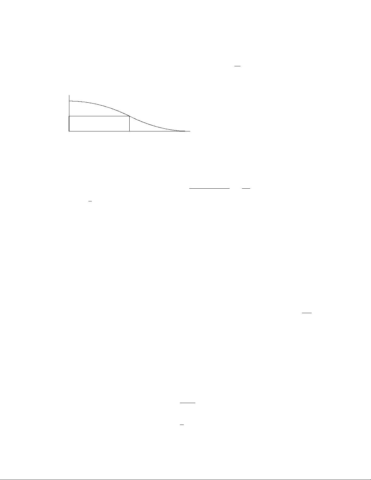
Area = a Pr(X ≥ a)
a
Pr(X ≥ a)
a Pr(X ≥ a) ≤
∞
0
Pr(X ≥ x) dx = E[X].
(d) As the hint says, let X =(Y −E[Y ])
2
. Then for any a ≥ 0,
Pr{(Y −E[Y ])
2
≥ a) ≤
E[(Y −E[Y ])
2
a
=
σ
2
Y
a
.
Letting b =
√
a completes the derivation.
Exercise 2.4:
(a) Since X
1
and X
2
are iid, symmetry implies that Pr(X
1
>X
2
) = Pr(X
2
>X
1
). These two
events are mutually exclusive and the event X
1
= X
2
has 0 probability. Thus Pr(X
1
>X
2
) and
Pr(X
1
<X
2
) sum to 1, so must each be 1/2. Thus Pr(X
1
≥ X
2
) = Pr(X
2
≥ X
1
)=1/2.
(b) Invoking the symmetry among X
1
, X
2
and X
3
, we see that each has the same probability of
being the smallest of the three (the probability of a tie is 0). These three events are mutually
exclusive and their probabilities must add up to 1. Therefore each event occurs with probability
1/3.
(c) The event {N>n} is the same as the event {X
1
is the minimum among the n iid
random variables X
1
, X
2
, ···, X
n
}. By extending the argument in part (b), we see that
Pr(X
1
is the smallest of X
1
,... ,X
n
)=1/n. Finally, Pr {N ≥ n} =Pr{N>n− 1}=
1
n−1
for
n ≥ 2.
(d) Since N is a non-negative integer random variable (taking on values from 2 to ∞), we can
use Exercise 2.3(a) as follows:
E[N]=
∞
n=1
Pr {N ≥ n}
=Pr{N ≥ 1} +
∞
n=2
Pr {N ≥ n}
=1+
∞
n=2
1
n − 1
=1+
∞
n=1
1
n
.
4

Since the series
∞
n=1
1
n
diverges, we conclude that E[N]=∞.
(e) Since the alphabet has a finite number of letters,
1
Pr(X
1
= X
2
) is no longer 0 and depends
on the particular probability distribution. Thus, although, Pr(X
1
≥ X
2
) = Pr(X
2
≥ X
1
)by
symmetry, neither can be found without knowing the distribution.
Out of the alphabet letters with nonzero probability, let a
min
be a letter of minimum numeric
value. If X
1
= a
min
, then no subsequent rv X
2
,X
3
,... can have a smaller value, so N = ∞ in
this case. Since the event X
1
= a
min
occurs with positive probability, E[N]=∞.
Exercise 2.5: First observe that for any n ≥ 1, the number of binary n-tuples with an even
number of 1’s is equal to the number of binary n-tuples with an odd number of 1’s. To see
this, note that for each sequence (x
1
,x
2
, ··· ,x
n−1
, 0), there corresponds a unique sequence
(x
1
,x
2
, ··· ,x
n−1
, 1). One of these two sequences has an odd number of 1’s while the other has
an even number of 1’s.
Since all 2
n
n-sequences are equally likely, the probability of an even number of ones then equals
the probability of an odd number, i.e.,
Pr(X
1
⊕ X
2
⊕···⊕X
n
= 0) = Pr(X
1
⊕ X
2
⊕···⊕X
n
=1) =
1
2
.
(a) Since Z = X
1
⊕···⊕X
n
, this shows that the binary random variable Z takes on the values
0 and 1 with equal probability. Now, conditional on X
1
=0,Z will be 0 if X
2
⊕···⊕X
n
=0,
which, from above (using X
2
... ,X
n
in place of X
1
,... ,X
n
) has probability 1/2. Similarly,
conditional on X
1
=1,Z again takes on the values 0 and 1 with probability 1/2 each. Thus Z
is independent of X
1
.
(b) Given that X
1
= x
1
,X
2
= x
2
, ··· ,X
n−1
= x
n−1
, Z is equal to 0 if X
n
= x
1
⊕x
2
⊕···⊕x
n−1
.
Since X
n
is independent of X
1
,... ,X
n−1
, and is equiprobably 0 or 1, it follows that Z =0
under this conditioning with probability 1/2 and Z = 1 with probability 1/2. Since this is true
for all choices of x
1
,... ,x
n−1
it follows that Z is independent of X
1
,... ,X
n−1
.
(c) Z, X
1
,X
2
, ··· ,X
n
are NOT statistically independent, and in fact, Z is uniquely determined
by X
1
,... ,X
n
.
(d) Z is NOT statistically independent of X
1
if Pr(X
i
=1)=p =1/2. We demonstrate this for
n = 2. The conditional PMF p
Z|X
1
(z|x
1
) for x
1
= 0 and 1 is
p
Z|X
1
(0|0) = Pr(X
2
=0)=1− p,
p
Z|X
1
(0|1) = Pr(X
2
=1)=p.
Since the conditional PMF for Z depends on X
1
, Z and X
1
are statistically dependent.
The purpose of this question is to show that in a group of n+1 random variables, pairwise
statistical independence (part a) does not imply statistical independence of all the random
variables (part c) (even with the statistical independence of groups of n random variables in
part (b).
1
The same results can be obtained with some extra work for a countably infinite discrete alphabet.
5


