没有合适的资源?快使用搜索试试~ 我知道了~
资源推荐
资源详情
资源评论
Ensemble Tracking
Shai Avidan
Abstract—We consider tracking as a binary classification problem, where an ensemble of weak classifiers is trained online to
distinguish between the object and the background. The ensemble of weak classifiers is combined into a strong classifier using
AdaBoost. The strong classifier is then used to label pixels in the next frame as either belonging to the object or the background, giving
a confidence map. The peak of the map and, hence, the new position of the object, is found using mean shift. Temporal coherence is
maintained by updating the ensemble with new weak classifiers that are trained online during tracking. We show a realization of this
method and demonstrate it on several video sequences.
Index Terms—AdaBoost, visual tracking, video analysis, concept learning.
Ç
1INTRODUCTION
V
ISUAL tracking is a critical step in many machine vision
applications such as surveillance [22], driver assistance
systems [1], or human-computer interactions [3]. Tracking
finds a region in the current image that matches the given
object, but if the matching function takes into account only
the object, and not the background, then it might not be able
to correctly distinguish the object from the background and
the tracking might fail.
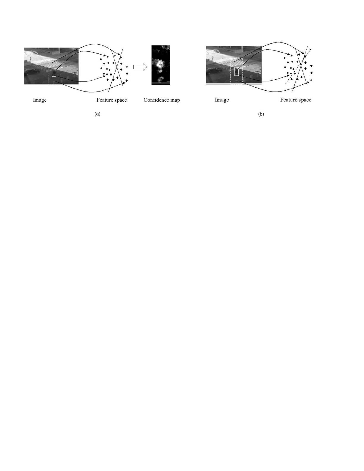
We treat tracking as a classification problem and train a
classifier to distinguish the object from the background.
This is done by constructing a feature vector for every pixel
in the reference image and training a classifier to separate
pixels that belong to the object from pixels that belong to the
background. Given a new video frame, we use the classifier
to test the pixels and form a confidence map. The peak of
the map is where we believe the object moved to and we
use mean shift [6] to find it.
If the object and background do not change over time,
then training a classifier when the tracker is initialized
would suffice, but, when the object and background change
their appearance, then the tracker must adapt accordingly.
Temporal integration is maintained by constantly training
new weak classifiers and adding them to the ensemble of
weak classifiers. The ensemble thus achieves two goals:
Each weak classifier is tuned to separate the object from the
background in a particular frame and the ensemble as a
whole ensures temporal coherence.
The overall algorithm proceeds as follows: We maintain an
ensemble of weakclassifiers that is used to create a confidence
map of the pixels in the current frame and run mean-shift to
find its peak and, hence, the new position of the object. Then,
we update the ensemble by training a new weak classifier on
the current frame and adding it to the ensemble.
Ensemble tracking extends traditional mean-shift tracking
in a number of important directions. First, mean-shift
tracking usually works with histograms of RGB colors. This
is because gray-scale images do not provide enough informa-
tion for tracking and high-dimensional feature spaces cannot
be modeled with histograms due to exponential memory
requirements. By switching to general machine learning
classifiers, ensemble tracking avoids both pitfalls. It can
handle gray-scale images by introducing local neighborhood
information and it does not suffer from exponential memory
explosion because it is no longer restricted to working with
histograms, as it can work with any type of classifier. Second,
ensemble tracking gives a principled manner in which the
classifiers are integrated over time. This is in contrast to
existing methods that either represent the foreground object
using the most recent histogram or some ad hoc combination
of the histograms of the first and last frames.
In addition, the proposed method offers several advan-
tages. It breaks the time consuming training phase into a
sequence of simple and easy to compute learning tasks that
can be performed online. It can automatically adjust the
weights of different classifiers, trained on different feature
spaces. It can also integrate offline and online learning
seamlessly. For example, if the object class to be tracked is
known, then one can train several weak classifiers offline on
large data sets and use these classifiers in addition to the
classifiers learned online. Also, integrating classifiers over
time improves the stability of the tracker in cases of partial
occlusions or illumination changes. Finally, on a higher
level, one can view ensemble tracking as a method for
training classifiers on time-varying distributions.
2BACKGROUND
Ensemble learning techniques combine a collection of weak
classifiers into a single strong classifier. AdaBoost [13], for
example, trains a weak classifier on increasingly more
difficult examples and combines the result to produce a
strong classifier that is better than any of the weak classifiers.
Treating tracking as a binary classification problem was
already considered in the past. Lin et al. [20] suggest an
adaptive discriminative generative model where a Fisher
Linear Discriminant function is const antly evaluated to
discri minate the object from the back ground. A similar
approach was taken by Nguyen and Smeulders [21].
Comaniciu et al. [6] adopt this approach to their mean-shift
algorithm, where colors that appear on the object are
IEEE TRANSAC TIONS ON PATTERN ANALYSIS AND MACHINE INTELLIGENCE, VOL. 29, NO. 2, FEBRUARY 2007 261
. The author is with Mitsubishi Electric Research Labs, 201 Broadway,
Cambridge, MA 02139. E-mail: avidan@merl.com.
Manuscript received 3 Nov. 2005; revised 14 Apr. 2006; accepted 18 May
2006; published online 13 Dec. 2006.
Recommended for acceptance by P. Fua.
For information on obtaining reprints of this article, please send e-mail to:
tpami@computer.org, and reference IEEECS Log Number TPAMI-0600-1105.
0162-8828/07/$20.00 ß 2007 IEEE Published by the IEEE Computer Society
down-weighted by colors that appear in the background. This
was further extended by Collins et al. [5], who were the first to
treat tracking as a binary classification problem, use online
feature selection to switch to the most discriminative color
space from a set of different color spaces.
Temporal integration methods include particle filtering
[16] to properly integrate measurements over time, the
WSL tracker [17] that maintains short-term and long-term
object descriptors that are constantly updated and re-
weighted using online-EM, and the incremental subspace
approach [15] in which an adaptive subspace is constantly
updated to maintain a robust and stable object descriptor.
It is instructive to compare these methods to ours. The
WSL and incremental subspace methods can be viewed as
generative methods that aim to explain the foreground object
while ignoring the background. Also, these methods are
template-based, meaning that they maintain the spatial
integrity of the object and, thus, are especially suited for
handling rigid objects. Ensemble tracking, on the other hand,
maintains an implicit representation of the foreground and
the background through the use of the classifiers. In addition,
ensemble tracking works on a pixel level, so global spatial
relationships are not maintained. This is useful when the
object deforms or undergoes severe appearance changes.
Particle filtering maintains a probability distribution function
over state space (i.e., what are the locations where the object
can be and what are the probabilities associated with each
such hypothesis). This means that particle filtering can be
used in conjunction with ensemble tracking, where the latter
is used to form the measurements (i.e., the confidence map)
that are used by the former.
A similar problem, termed “concept drift,” is considered
in the data mining literature where the goal is to quickly
scan large volumes of data and learn a concept (“object” in
computer vision jargon). As the concept might drift, the
classifier must adapt as well. For example, [18] presents
“dynamic weighted majority” as a method to track concept
drift for data mining applications, while [4] adds change
detection to concept drift to detect abrupt changes in the
concept, much in the spirit of the WSL tracker [17].
The work most closely related to ours is that of [5], which
uses online feature selection to find the best feature space to
work in. We extend this work in a number of important
ways. First, our classification framework automatically
weights the different features, as opposed to the discrete
nature of feature selection. Second, we depart from
histograms as the means for generating the confidence
map for mean-shift, meaning we can work with high-
dimensional feature spaces as opposed to the low-dimen-
sional feature spaces often used in the mean-shift literature.
Finally, our ensemble tracking technique gives a general
way of adaptively building discriminant functions over
time varying distributions.
3ENSEMBLE TRACKING
Ensemble tracking constantly updates a collection of weak
classifiers to separate the foreground object from the back-
ground. The weak classifiers can be added or removed at any
time to reflect changes in object appearance or incorporate
new information about the background. Hence, we do not
represent an object explicitly, instead we use an ensemble of
classifiers to determine if a pixel belongs to the object or not.
Each weak classifier is trained on positive and negative
examples where, by convention, we term examples coming
from the object as positive examples and examples coming
from the background as negative examples. The strong
classifier, calculated using AdaBoost, is then used to classify
the pixels in the next frame, producing a confidence map of
the pixels, where the classification margin is used as the
confidence measure. The peak of the map is where we believe
the object is and we use mean shift to find it. Once the
detection for the current frame is completed, we train a new
weak classifier on the new frame, add it to the ensemble, and
repeat the process all over again. Fig. 1 gives an overview of
the system. A general algorithm is given in Algorithm 1.
Another way to look at ensemble tracking is to consider
it as a method for building, and maintaining, a discriminant
function over time varying distributions. In this case, we
deal with distributions of object and background pixels, but
ensemble tracking can be used in other scenarios as well.
Our method constructs an ensemble classifier online.
This begs the question of what guarantees, if any, do we
have on its errors over the training set as well as its
generalization error. AdaBoost assumes a static distribution
and an access to a weak learner that performs better than
chance on this distribution. Ensemble tracking, on the other
hand, assumes time-varying distributions. However, be-
cause we are dealing with video, we assume that the
distribution changes slowly, so past weak classifiers still
262 IEEE TRANSACTIONS ON PATTERN ANALYSIS AND MACHINE INTELLIGEN CE, VOL. 29, NO. 2, FEBRUARY 2007
Fig. 1. Ensemble update and test. (a) The pixels of image at time t 1 are mapped to a feature space (circles for positive examples and crosses for
negative examples). Pixels within the solid rectangle are assumed to belong to the object, pixels outside the solid rectangle and within the dashed
rectangle are assumed to belong to the background. The examples are classified by the current ensemble of weak classifiers (denoted by the two
separating hyperplanes). The ensemble output is used to produce a confidence map that is fed to the mean shift algorithm. (b) Now, we train a new
weak classifier (the dashed line) on the pixels of the image at time t and add it to the ensemble.
perform better than chance on the new data, which gives
error bounds on the test error of ensemble tracking. In
practice, AdaBoost was shown to perform much better than
predicted by the theoretical analysis and we found the same
to be true with our ensemble tracking algorithm.
Algorithm 1 General Ensemble Tracking
Input: n video frames I
1
; ...;I
n
Rectangle r
1
of object in first frame
Output: Rectangles r
2
; ...;r
n
Initialization (for frame I
1
):
. Trai n T wea k classif iers and add them to the
ensemble.
For each new frame I
j
do:
. Test all pixels in frame I
j
using the current strong
classifier and create a confidence map L
j
.
. Run mean shift on the confidence map L
j
and report
new object rectangle r
j
.
. Label pixels inside rectangle r
j
as object and all those
outside it as background.
. Keep K “best” weak classifiers.
. Train new T K weak classifiers on frame I
j
and
add them to the ensemble.
3.1 The Wea k Classifier
The ensemble tracking framework is a general framework
that can be implemented in different ways. We report the
particular decisions we made in our system.
Let each pixel be represented as a d-dimensional feature
vector that consists of some local information and let
fx
i
;y
i
g
N
i¼1
denote N examples and their labels, respectively,
where x
i
2R
d
and y
i
2f1; þ1g. The weak classifier is
given by hðxÞ : R
d
!f1; þ1g, which is defined as:
hðxÞ¼signðh
T
xÞ;
where h 2R
d
is a separating hyperplane that is computed
using weighted least square regression
h ¼ðA
T
W
T
WAÞ
1
A
T
W
T
Wy:
Each row of the matrix A, denoted A
i
, corresponds to
one example x
i
augmented with the constant 1, that is A
i
¼
½x
i
; 1 and W is a diagonal matrix of the weights. We found
it useful to scale the sum of weights of positive, as well as
negative, examples to be equal to 0.5. This prevents bias to
the negative examples if the area of the object is smaller
than that of the background.
The temporal coherence of video is exploited by main-
taining a list of T classifiers that are trained over time. In each
frame, we keep the K “best” weak classifiers, discard the
remaining T K weak classifiers, train T K new weak
classifiers on the newly available data, and reconstruct the
strong weak classifier.
Prior knowledge about the object to be tracked can be
incorporated into the tracker in the form of one or more
weak classifiers that participate in the strong classifier, but
cannot be removed in the update stage.
Here, we use the same feature space across all classifiers,
but this does not have to be the case. Fusing various cues [7],
[8] was proven to improve tracking results and ensemble
tracking provides a flexible framework to do so.
The margin of the weak classifier hðxÞ is mapped to a
confidence measure cðxÞ by clipping negative margins to
zero and rescaling the positive margins to the range [0, 1].
The confidence value is then used in the confidence map
that is fed to the mean shift algorithm. The specific
algorithm we use is given in Algorithm 2.
3.2 Ensemble Update
In the update state, the algorithm keeps the “best” K weak
classifiers, thus making room for T K new weak classifiers.
However, before adding the new weak classifiers one needs
to update the weight of the remaining K weak classifiers. This
is done in Step 7 of Algorithm 2. Instead of training a new
weak classifier, the weak learner simply hands AdaBoost one
weak classifier (from the existing set of T weak classifiers) at a
time. By repeating this process K times, we effectively choose
the best K weak classifiers from the current ensemble of
T classifiers. This saves training time and creates a strong
classifier as well as a sample distribution that can be used for
training the new weak classifier, as is done in Step 8.
Care must be taken when adding or reweighting a weak
classifier that does not perform much better than chance. If,
during weight recalculation, the weak classifier performs
worse than chance, then we set its weight to zero. During
Step 8, we require the new weak classifier to perform
significantly better than chance. Specifically, we abort the
loop in Step 8 of the steady state in Algorithm 2 if err,
calculated in Step 8c, is above some threshold, which is set
to 0.4 in our case. This is especially important in case of
occlusions or severe illumination artifacts where the weak
classifier might learn data that does not belong to the object
but rather to the occluding object or to the illumination.
Algorithm 2 Specific Ensemble Tracking
Input: n video frames I
1
; ...;I
n
Rectangle r
1
of object in first frame
Output: Rectangles r
2
; ...;r
n
Initialization (for frame I
1
):
1) Extract fx
i
g
N
i¼1
examples with labels fy
i
g
N
i¼1
.
2) Initialize weights fw
i
g
N
i¼1
to be
1
N
.
3) For t ¼ 1...T ,
a) Make fw
i
g
N
i¼1
a distribution.
b) Train weak classifier h
t
.
c) Set err ¼
P
N
i¼1
w
i
jh
t
ðx
i
Þy
i
j.
d) Set weak classifier weight
t
¼
1
2
log
1err
err
e) Update example weights w
i
¼ w
i
e
ð
t
jh
t
ðx
i
Þy
i
jÞ
.
4) The strong classifier is given by signðHðxÞÞ, where
HðxÞ¼
P
T
t¼1
t
h
t
ðxÞ.
For each new frame I
j
do:
1) Extract fx
i
g
N
i¼1
examples.
2) Test the examples using the strong classifier HðxÞ
and create confidence image L
j
.
3) Run mean-shift on L
j
with r
j1
as the initial guess.
Let r
j
be the result of the mean shift algorithm.
4) Define labels fy
i
g
N
i¼1
with respect to the new
rectangle r
j
.
5) Keep best K weak classifiers.
6) Initialize weights fw
i
g
N
i¼1
to be
1
N
.
AVIDAN: ENSEMBLE TRACKING 263
剩余10页未读,继续阅读
资源评论
- hustasdfasdf2013-12-22ensemble Tracking的论文,英文,难理解。
dragon_perfect
- 粉丝: 298
- 资源: 20
上传资源 快速赚钱
- 我的内容管理 展开
- 我的资源 快来上传第一个资源
- 我的收益 登录查看自己的收益
- 我的积分 登录查看自己的积分
- 我的C币 登录后查看C币余额
- 我的收藏
- 我的下载
- 下载帮助
最新资源
- Python爬取淘宝热卖商品并可视化分析
- 5152单片机proteus仿真和源码将按键次数写入AT24C02再读出并用1602LCD显示
- SE-SSD复现过程(Det3D的安装教程)
- 基于Python的在线学习与推荐系统设计与实现(论文+源码)-kaic
- 串口通过 YMODEM 协议进行文件传输
- 蓝桥杯2024年第十五届省赛真题-前缀总分
- com.qihoo.appstore_300101305-1.apk
- tensorflow-gpu-2.7.1-cp37-cp37m-manylinux2010-x86-64.whl
- tensorflow-2.7.2-cp37-cp37m-manylinux2010-x86-64.whl
- tensorflow-2.7.1-cp39-cp39-manylinux2010-x86-64.whl
资源上传下载、课程学习等过程中有任何疑问或建议,欢迎提出宝贵意见哦~我们会及时处理!
点击此处反馈
安全验证
文档复制为VIP权益,开通VIP直接复制
信息提交成功