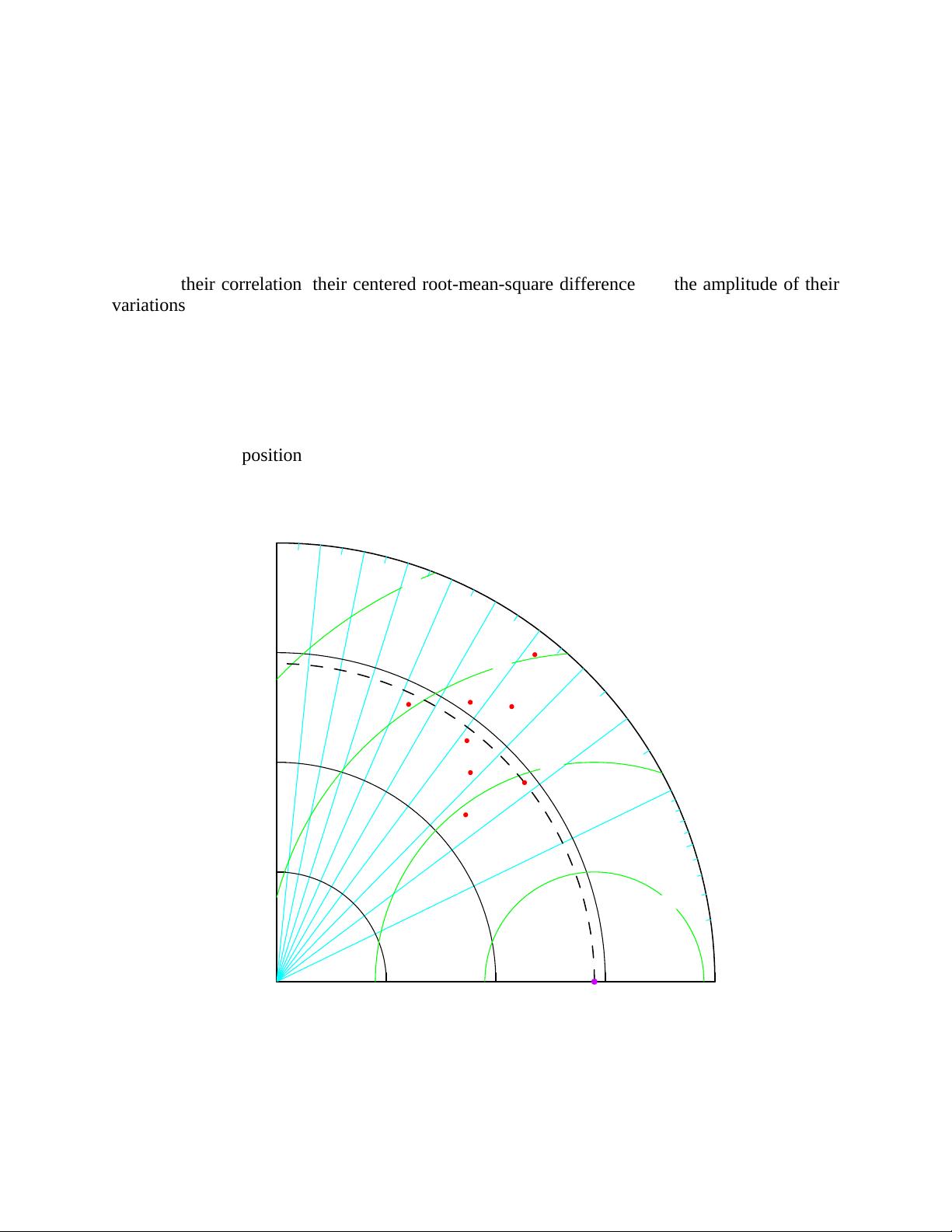
pattern correlation with observations is about 0.65. The centered root-mean-square (RMS)
difference between the simulated and observed patterns is proportional to the distance to the
point on the x-axis identified as "observed." The green contours indicate the RMS values and it
can be seen that in the case of model F the centered RMS error is about 2.6 mm/day. The
standard deviation of the simulated pattern is proportional to the radial distance from the origin.
For model F the standard deviation of the simulated field (about 3.3 mm/day) is clearly greater
than the observed standard deviation which is indicated by the dashed arc at the observed value
of 2.9 mm/day.
The relative merits of various models can be inferred from figure 1. Simulated patterns that
agree well with observations will lie nearest the point marked "observed" on the x-axis. These
models will have relatively high correlation and low RMS errors. Models lying on the dashed
arc will have the correct standard deviation (which indicates that the pattern variations are of the
right amplitude). In figure 1 it can be seen that models A and C generally agree best with
observations, each with about the same RMS error. Model A, however, has a slightly higher
correlation with observations and has the same standard deviation as the observed, whereas
model C has too little spatial variability (with a standard deviation of 2.3 mm/day compared to
the observed value of 2.9 mm/day). Of the poorer performing models, model E has a low pattern
correlation, while model D has variations that are much larger than observed, in both cases
resulting in a relatively large (~3 mm/day) centered RMS error in the precipitation fields. Note
also that although models D and B have about the same correlation with observations, model B
simulates the amplitude of the variations (i.e., the standard deviation) much better than model D,
and this results in a smaller RMS error.
In general, the Taylor diagram characterizes the statistical relationship between two fields, a
"test" field (often representing a field simulated by a model) and a "reference" field (usually
representing “truth”, based on observations). Note that the means of the fields are subtracted out
before computing their second-order statistics, so the diagram does not provide information
about overall biases, but solely characterizes the centered pattern error.
The reason that each point in the two-dimensional space of the Taylor diagram can represent
three different statistics simultaneously (i.e., the centered RMS difference, the correlation, and
the standard deviation) is that these statistics are related by the following formula:
RE
rfrf
σσσσ
2
22
2
−+=
′
,
where R is the correlation coefficient between the test and reference fields, E' is the centered
RMS difference between the fields, and σ
f
2
and σ
r
2
are the variances of the test and reference
fields, respectively. (The formulas for calculating these second order statistics are provided at
the end of this document.) The construction of the diagram (with the correlation given by the
cosine of the azimuthal angle) is based on the similarity of the above equation and the Law of
Cosines:
φ
cos2
222
abbac −+=