HiddenMarkovMapMatchingThroughNoiseandSparseness.pdf_隐马尔可夫链如Dijkstra算法资源-CSDN文库

4星 · 超过85%的资源需积分: 50 139 浏览量 2016-05-14 15:25:40 上传评论收藏 843KB PDF 举报

资源推荐

资源详情

资源评论

Hidden Markov Map Matching

Through Noise and Sparseness

Paul Newson and John Krumm

Microsoft Research

Microsoft Corporation

One Microsoft Way

Redmond, WA 98052 USA

+1 425 705 4507, +1 425 703 8283

{pnewson, jckrumm}@microsoft.com

ABSTRACT

The problem of matching measured latitude/longitude points to

roads is becoming increasingly important. This paper describes a

novel, principled map matching algorithm that uses a Hidden

Markov Model (HMM) to find the most likely road route

represented by a time-stamped sequence of latitude/longitude

pairs. The HMM elegantly accounts for measurement noise and

the layout of the road network. We test our algorithm on ground

truth data collected from a GPS receiver in a vehicle. Our test

shows how the algorithm breaks down as the sampling rate of the

GPS is reduced. We also test the effect of increasing amounts of

additional measurement noise in order to assess how well our

algorithm could deal with the inaccuracies of other location

measurement systems, such as those based on WiFi and cell tower

multilateration. We provide our GPS data and road network

representation as a standard test set for other researchers to use in

their map matching work.

Categories and Subject Descriptors

I.5.1 [Computing Methodologies]: Pattern Recognition, --

Models (Statistical)

General Terms

Algorithms, Measurement.

Keywords

Map matching, road map, location, driving routes.

1. INTRODUCTION

Map matching is the procedure for determining which road a

vehicle is on using data from sensors. The sensors almost always

include GPS because of its nearly ubiquitous availability. Map

matching has been important for many years on in-vehicle

navigation systems which must determine which road a vehicle is

traversing in real time. More recently, map matching is becoming

important as vehicles are used as traffic probes for measuring road

speeds and building statistical models of traffic delays. These

models, in turn, can be used to find time-optimal driving routes

that avoid traffic jams. Data from such traffic probes has been

used in the commercial routing engines of Microsoft [6], Dash [7],

and Inrix [8]. Map matching is also growing in importance for

research in route prediction [11], interpreting GPS traces [1], and

activity recognition [14].

This paper makes three contributions to the research in map

matching. First, it presents a new map matching algorithm based

on the Hidden Markov Model (HMM). While the HMM has been

used before in map matching, e.g. by Hummel [9], our

formulation is novel in some important respects, detailed

subsequently. We place particular emphasis on maintaining a

principled approach to the problem while simultaneously making

the algorithm robust to location data that is both geometrically

noisy and temporally sparse. Our second contribution is a test of

our map matching algorithm where we vary the levels of noise

and sparseness of the sensed location data over a 50 mile urban

drive. Varying the amount of noise lets us intelligently speculate

about how map matching would work with less accurate location

Permission to make digital or hard copies of all or part of this work for

personal or classroom use is granted without fee provided that copies are

not made or distributed for profit or commercial advantage, and that

copies bear this notice and the full citation on the first page. To copy

otherwise, to republish, to post on servers or to redistribute to lists,

requires prior specific permission and/or a fee. ACM GIS '09 , November

6/09/11...$10.00.

actual path

Figure 1: Map matching consists of matching measured

locations (black dots) to the road network in order to

infer the vehicle’s actual path (light gray curve). Merely

matching to the nearest road is prone to mistakes.

sensors, like multilateration from cell towers and WiFi access

points. Varying the sampling rate shows the minimum amount of

data required for good map matching. This is important for

practitioners who must decide on how often their GPS receivers

should sample location data, which affects requirements for

memory and bandwidth. Our third contribution is that we make

our GPS data, ground truth, and road network representation

publicly available for other researchers to use in their map

matching work. We believe this is the first time that such a data

set has been made publicly available. Until now, all the work on

map matching used private data sets for testing, making it

impossible to objectively compare results from different

algorithms.

2. THE MAP MATCHING PROBLEM

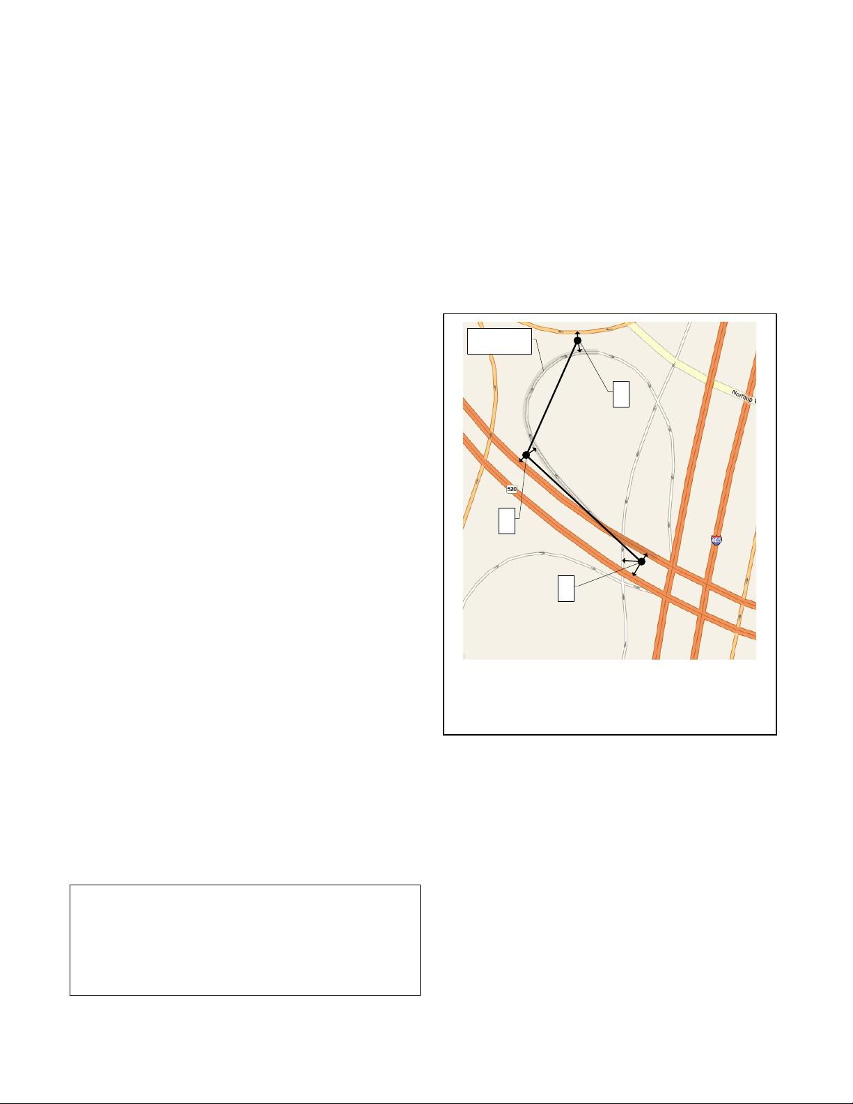
The map matching problem is illustrated in Figure 1. There are

three measured locations in sequence shown as black dots. The

problem is to find which roads the vehicle was on. The most

obvious algorithm is to simply match each point with the nearest

road. Due to measurement noise, however, this algorithm is prone

to error. In the illustration, the actual path is obvious, but the 2

and 3

point would be mismatched if they were associated with

the nearest road. Even using modern GPS receivers, we have

observed gross outliers and extended sequences of of erroneous

points, likely due to urban canyons and other terrestrial features

that affect GPS signals. Because of problems like this, modern

map matching takes into account sequences of points before

deciding on a match. In the example, there is really only one

reasonable path on the road network that could have produced the

observed measurements.

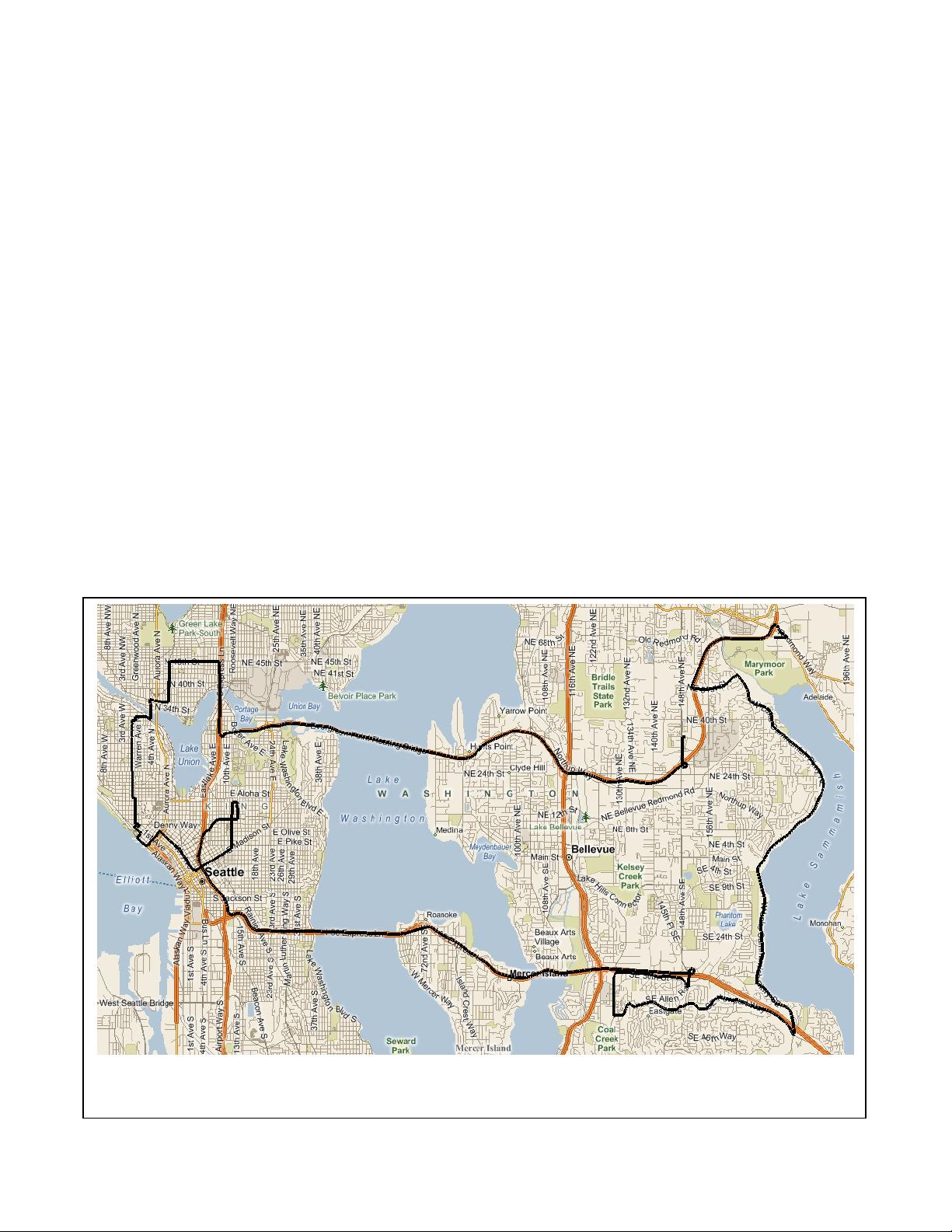
In our work, like most other map matching work, the raw input

data consists of vehicle locations measured by GPS, as shown in

Figure 2. Each measured point consists of a time-stamped

latitude/longitude pair. The roads are also represented in the

conventional way, as a graph of nodes and edges. The nodes are at

intersections, dead ends, and road name changes, and the edges

represent road segments between the nodes. Some edges are

directional to indicate one-way roads. Each node has an associated

latitude/longitude to indicate its location, and each edge has a

polyline of latitude/longitude pairs to represent its geometry.

Since point-by-point, nearest road matching often fails,

researchers have developed methods that match several points at

once. One way to do this is to create a (possibly smoothed) curve

from the location measurements and attempt to find matching

roads with similar geometry. As an example, White et al. [16]

present four algorithms, starting with the simple, nearest match

scheme. Their second algorithm adds orientation information to

the nearest match approach, comparing the measured heading to

the angle of the road. Their third algorithm evolves the second

algorithm to include connectivity constraints, and their fourth

algorithm does curve matching. They were surprised to discover

that their most sophisticated algorithm, the fourth one, was

outperformed by the simpler second algorithm when tested on a

total of about 17 km of driving data. Another purely geometric

approach comes from Greenfeld [5], whose algorithm builds up a

topologically feasible path through the road network. Matches are

determined by a similarity measure that weights errors based on

distance and orientation. The algorithm was found to perform

Figure 2: This is the GPS data we used for testing in the Seattle, Washington, USA area. The trip starts in the upper right near

Marymoor Park. It consists of 7531 GPS points sampled at 1 Hz, and it covers about 80 kilometers (50 miles) over about 2

hours.

剩余7页未读，继续阅读

评论收藏

内容反馈

z1198306833

2016-11-07

讲HMM在MM中应用的文章正在学习

河柚

粉丝: 2
资源: 14

Hidden Markov Map Matching Through Noise and Sparseness.pdf

最新资源

Hidden Markov Map Matching Through Noise and Sparseness.pdf

map-matching：基于GraphHopper的地图匹配

map_matching：找到车辆应该行驶以生成给定GPS轨迹的街道的算法

LeuvenMapMatching:Leuven.MapMatching工具箱，用于将GPS测量值与地图上的位置对齐

Markov Chains and Monte–Carlo Simulation.pdf

BERTifying the Hidden Markov Model for Multi-Source Weakly.pdf

论文研究-Markov 跳变系统输出峰值控制.pdf

A-Hidden Markov Model

A tutorial on hidden Markov models and selected applications in speech recognition

Nonlinear Markov Processes and Kinetic Equations.pdf

SUMS58 Understanding Markov Chains -- Examples and Applications.zip

Hidden-Markov-tree-model.rar_MARKOV_NOISE_hidden markov tree_mar

Wavelet-Based Statistical Signal Processing Using Hidden Markov Models，，，HMM

Hidden Markov Models for Time Series_An Introduction Using R (2nd Edition)

Markov Chain Monte Carlo and Gibbs Sampling.rar

Markov.Random.Field.Modeling.In.Image.Analysis.3rd.Edition

论文研究-基于Markov模型的动态电压调节策略.pdf

Image Analysis, Random Fields and Markov Chain Monte Carlo Methods.pdf

论文研究-基于Logistic-CA-Markov模型的用地变化动态模拟 .pdf

基于Markov链的分布式时间同步算法.pdf

Hidden Markov modelling.rar_Hidden Power_hidden markov_hidden vi

英文原版-Hidden Markov Models for Time Series 2nd Edition

网络攻击下的Markov跳变系统有限时间控制.pdf

转移概率一般不确知时滞Markov跳变神经网络的同步.pdf

最新资源