A-Hidden Markov Model
需积分: 13 106 浏览量
2019-02-26
17:39:46
上传
评论
收藏 566KB PDF 举报

Speech and Language Processing. Daniel Jurafsky & James H. Martin. Copyright
c
2018. All
rights reserved. Draft of September 11, 2018.
CHAPTER
A
Hidden Markov Models
Chapter 8 introduced the Hidden Markov Model and applied it to part of speech
tagging. Part of speech tagging is a fully-supervised learning task, because we have
a corpus of words labeled with the correct part-of-speech tag. But many applications
don’t have labeled data. So in this chapter, we introduce the full set of algorithms for
HMMs, including the key unsupervised learning algorithm for HMM, the Forward-
Backward algorithm. We’ll repeat some of the text from Chapter 8 for readers who
want the whole story laid out in a single chapter.
A.1 Markov Chains
The HMM is based on augmenting the Markov chain. A Markov chain is a model
Markov chain
that tells us something about the probabilities of sequences of random variables,
states, each of which can take on values from some set. These sets can be words, or
tags, or symbols representing anything, like the weather. A Markov chain makes a
very strong assumption that if we want to predict the future in the sequence, all that
matters is the current state. The states before the current state have no impact on the
future except via the current state. It’s as if to predict tomorrow’s weather you could
examine today’s weather but you weren’t allowed to look at yesterday’s weather.
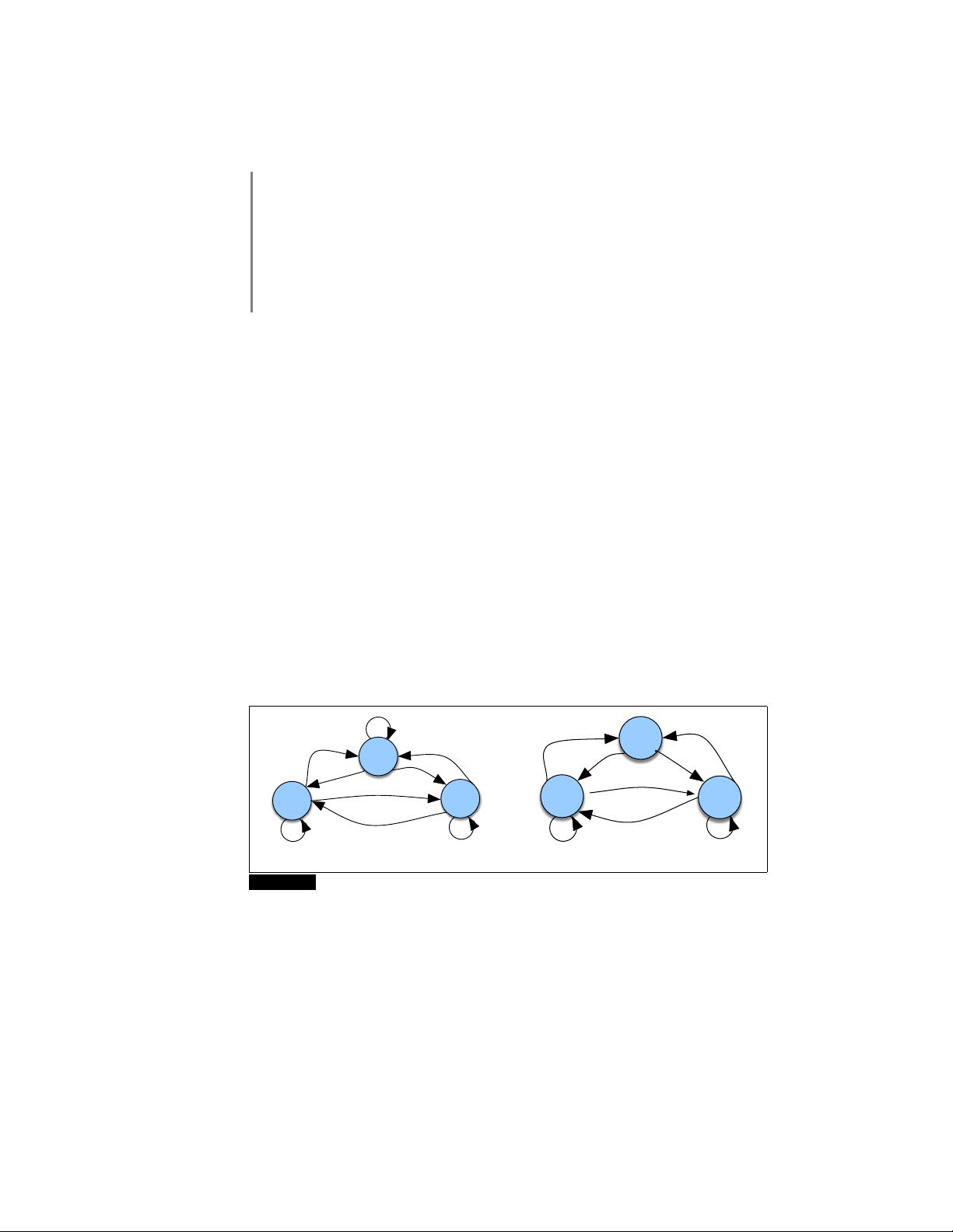
WARM
3
HOT
1
COLD
2
.8
.6
.1
.1
.3
.6
.1
.1
.3
charming
uniformly
are
.1
.4 .5
.5
.5
.2
.6 .2
(a) (b)
Figure A.1 A Markov chain for weather (a) and one for words (b), showing states and
transitions. A start distribution π is required; setting π = [0.1, 0.7, 0.2] for (a) would mean a
probability 0.7 of starting in state 2 (cold), probability 0.1 of starting in state 1 (hot), etc.
More formally, consider a sequence of state variables q
1
,q
2
,...,q
i
. A Markov
model embodies the Markov assumption on the probabilities of this sequence: that
Markov
assumption
when predicting the future, the past doesn’t matter, only the present.
Markov Assumption: P(q
i
= a|q
1
...q
i−1
) = P(q
i
= a|q
i−1
) (A.1)
Figure A.1a shows a Markov chain for assigning a probability to a sequence of
weather events, for which the vocabulary consists of HOT, COLD, and WARM. The
states are represented as nodes in the graph, and the transitions, with their probabil-
ities, as edges. The transitions are probabilities: the values of arcs leaving a given

剩余16页未读,继续阅读


评论0
最新资源