没有合适的资源?快使用搜索试试~ 我知道了~
CSE176 Introduction to Machine Learning — Lecture notes.pdf
需积分: 5 0 下载量 133 浏览量
2021-09-29
17:01:08
上传
评论
收藏 3.47MB PDF 举报
温馨提示
UCM《机器学习导论笔记》,80页pdf CSE176 Introduction to Machine Learning 从经验中学习的软件开发和分析技术综述。具体主题包括:监督学习(分类、回归);无监督学习(聚类、降维);强化学习;计算学习理论。具体的技术包括:贝叶斯方法、混合模型、决策树、基于实例的方法、神经网络、内核机器、集成等等。
资源推荐
资源详情
资源评论

CSE176 Introduction to Machine Learning — Lecture notes
Miguel
´
A. Carr eira-Perpi˜n´an
EECS, University of California, Merced
September 2, 2019
These are notes for a one-semester undergraduate course on machine learning given by Prof.
Miguel
´
A. Carreira-Perpi˜n´an at the University of California, Merced. The notes are largely based on
the book “Introduction to machine learning” by Ethem Alpaydın (MIT Press, 3rd ed., 2014), with
some additions.
These notes may be used for educational, no n-commercial purposes.
c
2015–2016 Miguel
´
A. Carreira-Perpi˜n´an

1 Introduction
1.1 What is machine learning (ML)?
• Data is being produced and stored continuously ( “big data”):
– science: genomics, astronomy, materials science, particle accelerators. . .
– sensor networ ks: weather measurements, traffic. . .
– people: social netwo r ks, blogs, mobile phones, purcha ses, bank tra nsactions. . .
– etc.
• Data is not r andom; it contains structure that can be used to predict outcomes, or gain knowl-
edge in some way.
Ex: patterns of Amazon purchases can be used to recommend items.
• It is more difficult t o design algor it hms for such tasks (compared to, say, sort ing an array or
calculating a payro ll) . Such algorithms need data.
Ex: construct a spam filter, using a collection of email messages labelled as spam/not s pam.
• Data mining: the application of ML methods to large databases.
• Ex of ML applications: f raud detection, medical diagnosis, speech or fa ce recognition. . .
• ML is programming computers using data (past experience) to optimize a performance criterion.
• ML relies on:
– Stat istics: making inferences from sample data.
– Numerical algorithms (linear alg ebra, opt imizatio n) : optimize criteria, manipulate models.
– Computer science: data structures and programs that solve a ML problem efficiently.
• A model:
– is a compressed version of a database;
– extracts knowledge from it;
– does not have perfect performance but is a useful approximation to the data.
1.2 Examples of ML problems
• Supervi s ed learning: labels provided.
– Classification (pattern recognition) :
∗ Face recognitio n. Difficult because of the complex variability in the data : pose and
illumination in a face ima ge, occlusions, glasses/beard/make-up/etc.
Training examples:
Test images:
∗ Optical character recognition: different styles, slant. . .
∗ Medical diagnosis: often, variables are missing (tests are costly).
1

∗ Speech recognition, machine translation, biometrics. . .
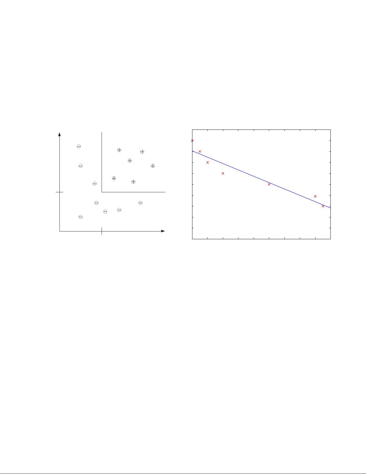
∗ Credit scoring: classify customers into high- and low-risk, based on their income and
savings, using data about past loans (whether they were pa id or not).
– Regres s i on: the labels to be predicted are continuous:
∗ Predict the price of a car from its mileage.
∗ Navigating a car: angle of the steering.
∗ Kinematics of a robot arm: predict wor kspace location from angles.
if income > θ
1
and savings > θ
2
then low-risk else high-risk
y = wx + w
0
Savings
Income
Low-Risk
High-Risk
θ
2
θ
1
x: mileage
y: price
• Unsupervised learning: no labels provided, only input data .
– Learning associations:
∗ Basket analysis: let p(Y |X) = “probability that a customer who buys product X
also buys product Y ”, estimated from past purchases. If p(Y |X) is large (say 0.7) ,
associate “X → Y ”. When someone buys X, recommend them Y .
– Clustering: group similar data points.
– D ensity estimation: where are data points likely to lie?
– D i mensionality reduction: data lies in a low-dimensional manifold.
– Feature selection: keep only useful features.
– Outlier/no velty detection.
• Semisupervised learning: labels provided for some points only.
• Reinf orcement learning: find a sequence o f actions (policy) that reaches a goal. No supervised
output but delayed reward.
Ex: playing chess or a computer game, robot in a m aze.
2

2 Supervised learning
2.1 Learning a class from examples: two-class prob lems
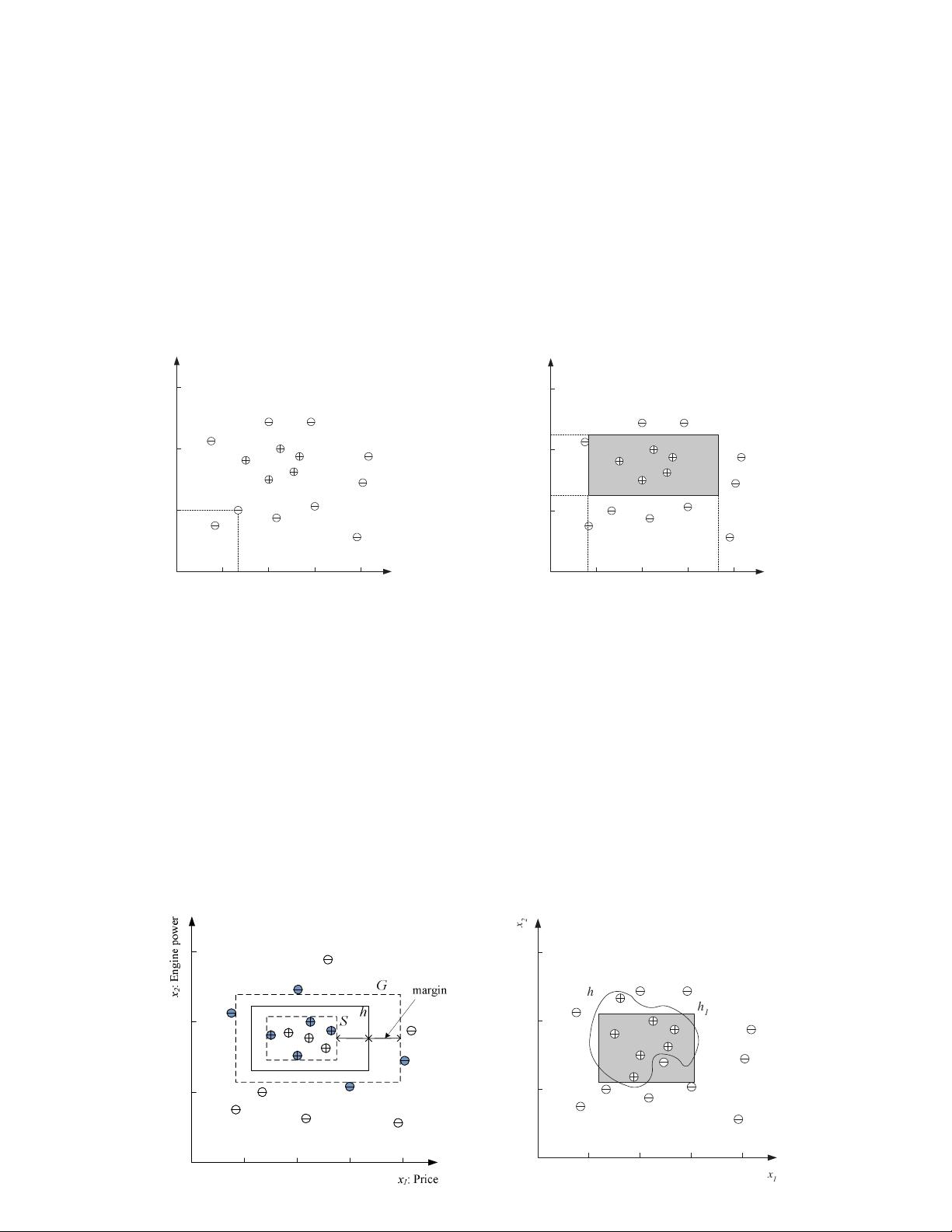
• We are given a training set of labeled examples (positive and negative) and want to learn a
classifier that we can use to predict unseen examples, or to understand the data.
• Input representation: we need to decide what attributes (features) to use to describe the input
patterns (examples, instances). This implies ignoring other attributes as irrelevant.
training set for a “family car”
Hypothesis class of rectangles
(p
1
≤ price ≤ p
2
) AND (e
1
≤ engine power ≤ e
2
)
where p
1
, p
2
, e
1
, e
2
∈ R
x
2
: Engine power
x
1
: Price
x
1
t
x
2
t
x
2
: Engine power
x
1
: Price
p
1
p
2
e
1
e
2
C
• Training set: X = {(x
n
, y
n
)}
N
n=1
where x
n
∈ R
D
is the nth input vector and y
n
∈ {0, 1} its
class label.
• Hypothesis (mod el) class
H: the set of classifier functions we will use. Idea lly, the true class
distribution C can be represented by a function in H (exactly, or with a small error).
• Having selected H, learning the class reduces to finding an optimal h ∈ H. We don’t know the
true class regions C, but we can approximate them by the empirical error:
E(h; X) =
N
X
n=1
I(h(x
n
) 6= y
n
) = number of misclassified instances
There may be more than one optimal h ∈ H. In that case, we achieve better generalization by maximizing the margin (the distance
between the boundary of h and the instances closest to it).
the hypothesis with the largest margin noise and a more complex hypothesis
x
2
x
1
h
1
h
2
3

2.4 Noise
• Noise is any unwanted anomaly in the data. It can be due to:
– Imprecision in recording the input attributes: x
n
.
– Errors in labeling the input vectors: y
n
.
– Attributes not considered that affect the label (h i dden or latent attributes, may be unob-
servable).
• Noise makes learning harder.
• Should we keep t he hypothesis class simple rather than complex?
– Easier to use and to train (fewer parameters, faster).
– Easier to explain or interpret.
– Less variance in the learned model than for a complex model (less affected by single
instances), but also higher bias.
Given compar able empirical error , a simple model will generalize better than a complex one.
(Occam’ s razor: simpler explanations are more plausible; eliminate unnecessary complexity.)
2.5 Learning multiple classes
• With K classes, we can code the label as a n integer y = k ∈ {1, . . . , K}, or as a one-of-K
binary vector y = (y
1
, . . . , y
K
)
T
∈ {0, 1}
K
(containing a single 1 in position k).
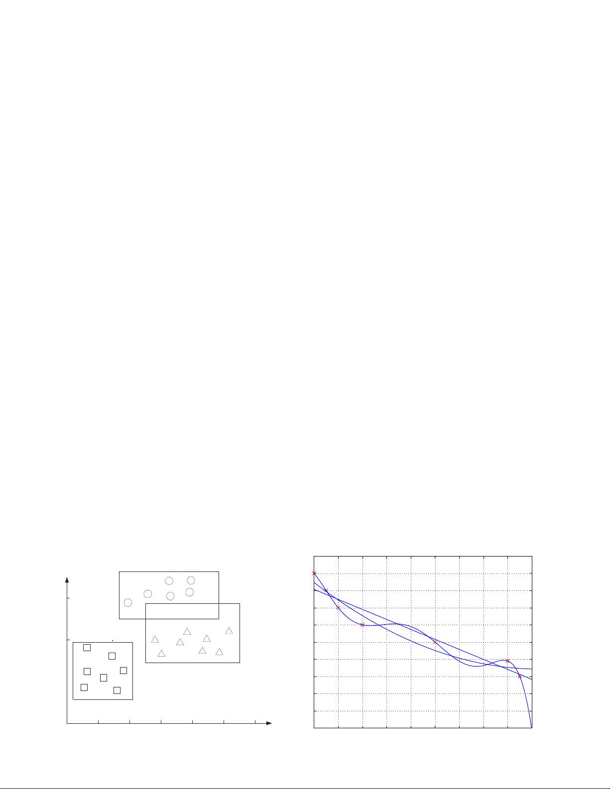
• One approach for K-class classification: consider it as K two-class classification problems, and
minimize the total empirical error:
E({h
k
}
K
k=1
; X) =
N
X
n=1
K
X
k=1
I(h
k
(x
n
) 6= y
nk
)
where y
n
is coded as o ne- of-K and h
k
is the two-class classifier for problem k, i.e., h
k
(x) ∈ {0, 1}.
• Ideally, for a given pattern x only one h
k
(x) is one. When no, or more than one, h
k
(x) is one
then the classifier is in doubt and may reject the pa t tern.
3-class example
regression: polynomials of order 1, 2, 6
(✐ solve for order 1: optimal w
0
, w
1
)
Engine power
Price
Family car
Sports car
Luxury sedan
?
?
x: milage
y: price
4
剩余79页未读,继续阅读
资源评论

努力+努力=幸运
- 粉丝: 4
- 资源: 136
上传资源 快速赚钱
 我的内容管理
展开
 我的资源
快来上传第一个资源
 我的收益 登录查看自己的收益
 我的积分
登录查看自己的积分
 我的C币
登录后查看C币余额
 我的收藏
我的收藏  我的下载
我的下载  下载帮助
下载帮助

 前往需求广场,查看用户热搜
最新资源
资源上传下载、课程学习等过程中有任何疑问或建议,欢迎提出宝贵意见哦~我们会及时处理!
点击此处反馈


安全验证
文档复制为VIP权益,开通VIP直接复制
 信息提交成功