Digital Image
Processing
Using MATLAB
®
Second Edition
Rafael C. Gonzalez
University of Tennessee
Richard E. Woods
MedData Interactive
Steven L. Eddins
The MathWorks, Inc.
Gatesmark Publishing
®
A Division of Gatesmark,
®
LLC
www.gatesmark.com

Library of Congress Cataloging-in-Publication Data on File
Library of Congress Control Number: 2009902793
© 2009 by Gatesmark, LLC
All rights reserved. No part of this book may be reproduced or transmitted in any form or by any
means, without written permission from the publisher.
Gatesmark Publishing
®
is a registered trademark of Gatesmark, LLC, www.gatesmark.com.
Gatesmark
®
is a registered trademark of Gatesmark, LLC, www.gatesmark.com.
MATLAB
®
is a registered trademark of The MathWorks, Inc., 3 Apple Hill Drive, Natick, MA
01760-2098
The authors and publisher of this book have used their best efforts in preparing this book. These
efforts include the development, research, and testing of the theories and programs to determine
their effectiveness. The authors and publisher shall not be liable in any event for incidental or
consequential damages with, or arising out of, the furnishing, performance, or use of these
programs.
Printed in the United States of America
10 9 8 7 6 5 4 3 2 1
ISBN 978-0-9820854-0-0
Gatesmark Publishing
A Division of Gatesmark, LLC
www.gatesmark.com
80
3
Intensity Transformations
and Spatial Filtering
Preview
The term spatial domain refers to the image plane itself, and methods in
this category are based on direct manipulation of pixels in an image. In this
chapter we focus attention on two important categories of spatial domain
processing: intensity (gray-level) transformations and spatial filtering. The lat-
ter approach sometimes is referred to as neighborhood processing, or spatial
convolution. In the following sections we develop and illustrate MATLAB
formulations representative of processing techniques in these two categories.
We also introduce the concept of fuzzy image processing and develop sever-
al new M-functions for their implementation. In order to carry a consistent
theme, most of the examples in this chapter are related to image enhancement.
This is a good way to introduce spatial processing because enhancement is
highly intuitive and appealing, especially to beginners in the field. As you will
see throughout the book, however, these techniques are general in scope and
have uses in numerous other branches of digital image processing.
3.1 Background
As noted in the preceding paragraph, spatial domain techniques operate di-
rectly on the pixels of an image. The spatial domain processes discussed in this
chapter are denoted by the expression
gxyTfxy(, )(,)=
[]
where
fxy(, )
is the input image,
gxy(, )
is the output (processed) image, and
T is an operator on f defined over a specified neighborhood about point
(, )xy
.
In addition, T can operate on a set of images, such as performing the addition
of K images for noise reduction.
3.2 ■ Background 81
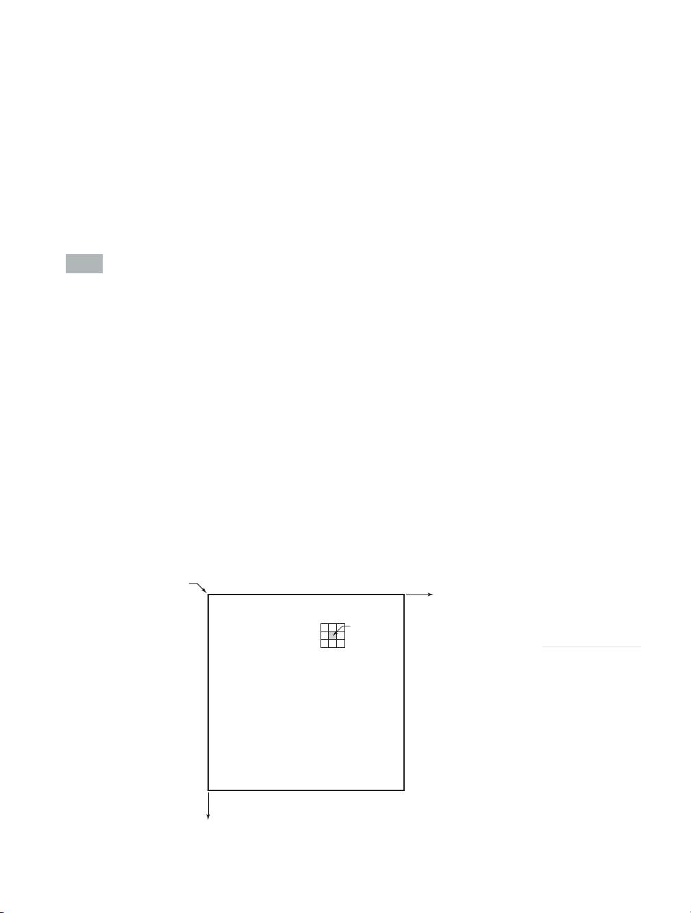
The principal approach for defining spatial neighborhoods about a point
(, )xy
is to use a square or rectangular region centered at
(, )xy
, as in Fig. 3.1. The center
of the region is moved from pixel to pixel starting, say, at the top, left corner,
and, as it moves, it encompasses different neighborhoods. Operator T is applied
at each location
(, )xy
to yield the output, g, at that location. Only the pixels in the
neighborhood centered at
(, )xy
are used in computing the value of g at
(, )xy
.
Most of the remainder of this chapter deals with various implementations
of the preceding equation. Although this equation is simple conceptually, its
computational implementation in MATLAB requires that careful attention be
paid to data classes and value ranges.
3.2 Intensity Transformation Functions
The simplest form of the transformation T is when the neighborhood in Fig. 3.1
is of size
11*
(a single pixel). In this case, the value of g at
(, )xy
depends only
on the intensity of f at that point, and T becomes an intensity or gray-level
transformation function. These two terms are used interchangeably when deal-
ing with monochrome (i.e., gray-scale) images. When dealing with color images,
the term intensity is used to denote a color image component in certain color
spaces, as described in Chapter 7.
Because the output value depends only on the intensity value at a point, and
not on a neighborhood of points, intensity transformation functions frequently
are written in simplified form as
sTr= ()
where r denotes the intensity of f and s the intensity of g, both at the same
coordinates
(, )xy
in the images.
y
x
Origin
(x, y)
Image f (x, y)
FIGURE 3.1
A neighborhood
of size
33*
centered at point
(, )xy
in an image.

82 Chapter 3 ■ Intensity Transformations and Spatial Filtering
3.2.1 Functions imadjust and stretchlim
Function imadjust is the basic Image Processing Toolbox function for inten-
sity transformations of gray-scale images. It has the general syntax
g = imadjust(f, [low_in high_in], [low_out high_out], gamma)
As Fig. 3.2 illustrates, this function maps the intensity values in image f to
new values in g, such that values between low_in and high_in map to values
between low_out and high_out. Values below low_in and above high_in
are clipped; that is, values below low_in map to low_out, and those above
high_in map to high_out. The input image can be of class uint8, uint16,
int16, single, or double, and the output image has the same class as the in-
put. All inputs to function imadjust, other than f and gamma, are specified as
values between 0 and 1, independently of the class of f. If, for example, f is of
class uint8, imadjust multiplies the values supplied by 255 to determine the
actual values to use. Using the empty matrix ([ ]) for [low_in high_in] or
for [low_out high_out] results in the default values [0 1]. If high_out is
less than low_out, the output intensity is reversed.
Parameter gamma specifies the shape of the curve that maps the intensity
values in f to create g. If gamma is less than 1, the mapping is weighted toward
higher (brighter) output values, as in Fig. 3.2(a). If gamma is greater than 1, the
mapping is weighted toward lower (darker) output values. If it is omitted from
the function argument, gamma defaults to 1 (linear mapping).
■ Figure 3.3(a) is a digital mammogram image, f, showing a small lesion, and
Fig. 3.3(b) is the negative image, obtained using the command
>> g1 = imadjust(f, [0 1], [1 0]);
This process, which is the digital equivalent of obtaining a photographic nega-
tive, is particularly useful for enhancing white or gray detail embedded in a
large, predominantly dark region. Note, for example, how much easier it is to
analyze the breast tissue in Fig. 3.3(b). The negative of an image can be ob-
tained also with toolbox function imcomplement:
imadjust
Recall from the
discussion in Section 2.7
that function
mat2gray
can be used for
converting an image to
class
double and scaling
its intensities to the
range [0, 1],
independently of the
class of the input image.
EXAMPLE 3.1:
Using function
imadjust.
low_in high_in
low_out
high_out
low_in high_inlow_in high_in
gamma 1 gamma 1 gamma 1
a b c
FIGURE 3.2
The various
mappings
available in
function
imadjust.