


Fundamentals of Image Processing
Ian T. Young
Jan J. Gerbrands
Lucas J. van Vliet

CIP-DATA KONINKLIJKE BIBLIOTHEEK, DEN HAAG
Young, Ian Theodore
Gerbrands, Jan Jacob
Van Vliet, Lucas Jozef
FUNDAMENTALS OF IMAGE PROCESSING
ISBN 90–75691–01–7
NUGI 841
Subject headings: Digital Image Processing / Digital Image Analysis
All rights reserved. No part of this publication may be reproduced, stored in a retrieval system, or
transmitted in any form or by any means—electronic, mechanical, photocopying, recording, or
otherwise—without the prior written permission of the authors.
Version 2.2
Copyright © 1995, 1997, 1998 by I.T. Young, J.J. Gerbrands and L.J. van Vliet
Cover design: I.T. Young
Printed in The Netherlands at the Delft University of Technology.

Fundamentals of Image Processing
1. Introduction..............................................1
2. Digital Image Definitions.........................2
3. Tools........................................................6
4. Perception...............................................22
5. Image Sampling.....................................28
6. Noise......................................................32
7. Cameras.................................................35
8. Displays.................................................44
Ian T. Young 9. Algorithms.............................................44
Jan J. Gerbrands 10. Techniques.............................................85
Lucas J. van Vliet 11. Acknowledgments...............................108
Delft University of Technology 12. References............................................108
1. Introduction
Modern digital technology has made it possible to manipulate multi-dimensional
signals with systems that range from simple digital circuits to advanced parallel
computers. The goal of this manipulation can be divided into three categories:
• Image Processing image in → image out
• Image Analysis image in → measurements out
• Image Understanding image in → high-level description out
We will focus on the fundamental concepts of image processing. Space does not
permit us to make more than a few introductory remarks about image analysis.
Image understanding requires an approach that differs fundamentally from the
theme of this book. Further, we will restrict ourselves to two–dimensional (2D)
image processing although most of the concepts and techniques that are to be
described can be extended easily to three or more dimensions. Readers interested in
either greater detail than presented here or in other aspects of image processing are
referred to [1-10]
We begin with certain basic definitions. An image defined in the “real world” is
considered to be a function of two real variables, for example, a(x,y) with a as the
amplitude (e.g. brightness) of the image at the real coordinate position (x,y). An
image may be considered to contain sub-images sometimes referred to as

…Image Processing Fundamentals
2
regions–of–interest, ROIs, or simply regions. This concept reflects the fact that
images frequently contain collections of objects each of which can be the basis for a
region. In a sophisticated image processing system it should be possible to apply
specific image processing operations to selected regions. Thus one part of an image
(region) might be processed to suppress motion blur while another part might be
processed to improve color rendition.
The amplitudes of a given image will almost always be either real numbers or
integer numbers. The latter is usually a result of a quantization process that converts
a continuous range (say, between 0 and 100%) to a discrete number of levels. In
certain image-forming processes, however, the signal may involve photon counting
which implies that the amplitude would be inherently quantized. In other image
forming procedures, such as magnetic resonance imaging, the direct physical
measurement yields a complex number in the form of a real magnitude and a real
phase. For the remainder of this book we will consider amplitudes as reals or
integers unless otherwise indicated.
2. Digital Image Definitions
A digital image a[m,n] described in a 2D discrete space is derived from an analog
image a(x,y) in a 2D continuous space through a sampling process that is
frequently referred to as digitization. The mathematics of that sampling process will
be described in Section 5. For now we will look at some basic definitions
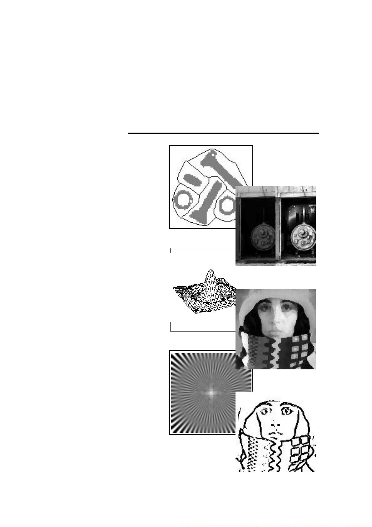
associated with the digital image. The effect of digitization is shown in Figure 1.
The 2D continuous image a(x,y) is divided into N rows and M columns. The
intersection of a row and a column is termed a pixel. The value assigned to the
integer coordinates [m,n] with {m=0,1,2,…,M–1} and {n=0,1,2,…,N–1} is a[m,n].
In fact, in most cases a(x,y)—which we might consider to be the physical signal
that impinges on the face of a 2D sensor—is actually a function of many variables
including depth (z), color (λ), and time (t). Unless otherwise stated, we will
consider the case of 2D, monochromatic, static images in this chapter.

…Image Processing Fundamentals
3
Rows
Columns
Value = a(x, y, z,
λ, t)
Figure 1: Digitization of a continuous image. The pixel at coordinates
[m=10, n=3] has the integer brightness value 110.
The image shown in Figure 1 has been divided into N = 16 rows and M = 16
columns. The value assigned to every pixel is the average brightness in the pixel
rounded to the nearest integer value. The process of representing the amplitude of
the 2D signal at a given coordinate as an integer value with L different gray levels is
usually referred to as amplitude quantization or simply quantization.
2.1 COMMON VALUES
There are standard values for the various parameters encountered in digital image
processing. These values can be caused by video standards, by algorithmic
requirements, or by the desire to keep digital circuitry simple. Table 1 gives some
commonly encountered values.
Parameter Symbol Typical values
Rows N 256,512,525,625,1024,1035
Columns M 256,512,768,1024,1320
Gray Levels L 2,64,256,1024,4096,16384
Table 1: Common values of digital image parameters
Quite frequently we see cases of M=N=2
K
where {K = 8,9,10}. This can be
motivated by digital circuitry or by the use of certain algorithms such as the (fast)
Fourier transform (see Section 3.3).


