量子零能条件，纠缠楔形嵌套和量子聚焦资源-CSDN文库

Open

Access

101 浏览量 2020-04-03 02:13:33 上传评论收藏 386KB PDF 举报

资源推荐

资源详情

资源评论

Quantum null energy condition, entanglement wedge nesting,

and quantum focusing

Chris Akers ,

Venkatesa Chandrasekaran,

†

Stefan Leichenauer,

‡

Adam Levine,

and Arvin Shahbazi Moghaddam

∥

Center for Theoretical Physics and Department of Physics,

University of California, Berkeley, California 94720, USA

and Lawrence Berkeley National Laboratory, Berkeley, California 94720, USA

(Received 14 November 2019; published 22 January 2020)

We study the consequences of entanglement wedge nesting for conformal field theories (CFTs) with

holographic duals. The CFT is formulated on an arbitrary curved background, and we include the effects of

curvature-squared couplings in the bulk. In this setup we find necessary and sufficient conditions for

entanglement wedge nesting to imply the quantum null energy condition in d ≤ 5, extending its earlier

holographic proofs. We also show that the quantum focusing conjecture yields the quantum null energy

condition as its nongravitational limit under these same conditions.

DOI: 10.1103/PhysRevD.101.025011

I. INTRODUCTION AND SUMMARY

The quantum focusing conjecture (QFC) is a new

principle of semiclassical quantum gravity proposed in

[1]. Its formulation is motivated by classical focusing,

which states that the expansion θ of a null congruence of

geodesics is nonincreasing. Classical focusing is at the

heart of several important results of classical gravity [2–5],

and likewise quantum focusing can be used to prove

quantum generalizations of many of these results [6–9].

One of the most important and surprising consequences of

the QFC is the quantum null energy condition (QNEC),

which was discovered as a particular nongravitational limit

of the QFC [1]. Subsequently the QNEC was proven for free

fields [10] and for holographic conformal field theories

(CFTs) on flat backgrounds [11] (and recently extended in

[12] in a similar way as we do here). The formulation of the

QNEC which naturally comes out of the proofs we provide

here is as follows.

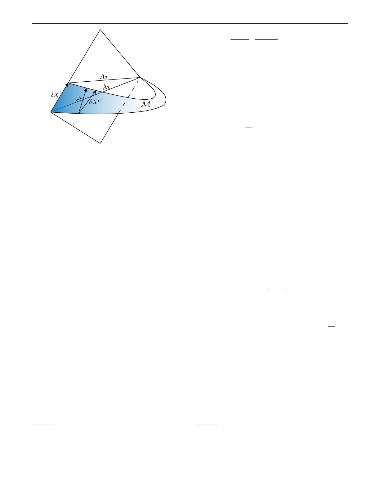
Consider a codimension-two Cauchy-splitting surface Σ ,

which we will refer to as the entangling surface. The Von

Neumann entropy S½Σ of the interior (or exterior) or Σ is a

functional of Σ, and in particular is a functional of the

embedding functions X

ðyÞ that define Σ. Choose a one-

parameter family of deformed surfaces ΣðλÞ, with

Σð0Þ¼Σ, such that (i) ΣðλÞ is given by flowing along

null geodesics generated by the null vector field k

normal

to Σ for affine time λ, and (ii) ΣðλÞ is either “shrinking” or

“growing” as a function of λ, in the sense that the domain of

dependence of the interior of Σ is either shrinking or

growing. Then for any point on the entangling surface we

can define the combination

ðyÞk

ðyÞ −

2π

dλ



ðyÞ

ﬃﬃﬃﬃﬃﬃﬃﬃﬃ

hðyÞ

δS

ren

δX

ðyÞ



: ð1:1Þ

Here

ﬃﬃﬃﬃﬃﬃﬃﬃﬃ

hðyÞ

is the induced metric determinant on Σ.

Writing this down in a general curved background requires

a renormalization scheme both for the energy-momentum

tensor T

and the renormalized entropy S

ren

. Assuming that

this quantity is scheme-independent (and hence well

defined), the QNEC states that it is positive. Our main

task is to determine the necessary and sufficient conditions

we need to impose on Σ and the background spacetime at

the point y in order that the QNEC hold.

In addition to a proof through the QFC, the holographic

proof method of [11] is easily adaptable to answering this

question in full generality. The backbone of that proof is

entanglement wedge nesting (EWN), which is a conse-

quence of subregion duality in AdS/CFT [9]. A given

region on the boundary of AdS is associated with a

particular region of the bulk, called the entanglement

wedge, which is defined as the bulk region spacelike-

related to the extremal surface [13–16] used to compute the

CFT entropy on the side toward the boundary region. This

bulk region is dual to the given boundary region, in the

sense that there is a correspondence between the algebras of

operators in the bulk region and the operators in the

boundary region which are good semiclassical gravity

cakers@berkeley.edu

†

ven_chandrasekaran@berkeley.edu

‡

sleichen@berkeley.edu

arlevine@berkeley.edu

∥

arvinshm@berkeley.edu

Published by the American Physical Society under the terms of

the Creative Commons Attribution 4.0 International license.

Further distribution of this work must maintain attribution to

the author(s) and the published article’s title, journal citation,

and DOI. Funded by SCOAP

PHYSICAL REVIEW D 101, 025011 (2020)

2470-0010=2020=101(2)=025011(21) 025011-1 Published by the American Physical Society

operators (i.e., they act within the subspace of semiclassical

states) [17–19]. EWN is the statement that nested boundary

regions must be dual to nested bulk regions, and clearly

follows from the consistency of subregion duality.

While the QNEC can be derived from both the QFC and

EWN, there has been no clear connection between these

derivations.

As it stands, there are apparently two QNECs,

the QNEC-from-QFC and the QNEC-from-EWN. We will

show in full generality that these two QNECs are in fact the

same, at least in d ≤ 5 dimensions.

Here is a summary of our results:

(i) The holographic proof of the QNEC from EWN is

extended to CFTs on arbitrary curved backgrounds.

In d ¼ 5 we find necessary that the necessary and

sufficient conditions for the ordinary QNEC to hold

at a point are that

ðkÞ

¼ σ

ðkÞ

¼ D

ðkÞ

¼ D

ðkÞ

¼ R

¼ 0 ð1:2Þ

at that point. For d<5 only a subset of these

conditions are necessary. This is the subject of

Sec. II C.

(ii) We also show holographically that under the weaker

set of conditions

ðkÞ

¼ D

ðkÞ

þ R

¼ D

ðkÞ

¼ 0 ð1:3Þ

the Conformal QNEC holds. The Conformal QNEC

was introduced in [11] as a conformally transformed

version of the QNEC. This is the strongest inequality

that we can get out of EWN. This is the subject of

Sec. II E

(iii) By taking the nongravitational limit of the QFC we

are able to derive the QNEC again under the same

set of conditions as we did for EWN. This is the

subject of § III B.

(iv) We argue in Sec. III C that the statement of the

QNEC is scheme-independent whenever the con-

ditions that allow us to prove it hold. This shows that

the two proofs of the QNEC are actually proving the

same, unambiguous field–theoretic bound.

We conclude in Sec. IV with a discussion and suggest

future directions. A number of technical Appendices are

included as part of our analysis.

A. Relation to other work

While this work was in preparation, [12] appeared

which has overlap with our discussion of EWN and the

scheme-independence of the QNEC. The results of [12]

relied on a number of assumptions about the background:

the null curvature condition and a positive energy con-

dition. From this they derive certain sufficient conditions

for the QNEC to hold. We do not assume anything about

our backgrounds a priori, and include all relevant higher

curvature corrections. This gives our results greater gen-

erality, as we are able to find both necessary and sufficient

conditions for the QNEC to hold.

II. ENTANGLEMENT WEDGE NESTING

A. Subregion duality

The statement of AdS/CFT includes a correspondence

between operators in the semiclassical bulk gravitational

theory and CFT operators on the boundary. Moreover, it has

been shown [19,20] that such a correspondence exists

between the operator algebras of subregions in the CFT and

certain associated subregions in the bulk as follows:

Consider a spatial subregion A in the boundary geometry.

The extremal surface anchored to ∂A, which is used to

compute the entropy of A [13,14], bounds the so-called

entanglement wedge of A, EðAÞ, in the bulk. More precisely

EðAÞ is the codimension-zero bulk region spacelike-related

to the extremal surface on the same side of the extremal

surface as A. Subregion duality is the statement that the

operator algebras of DðAÞ and EðAÞ are dual, where DðAÞ

denotes the domain of dependence of A

1. Entanglement wedge nesting

The results of this section follow from EWN, which we

now describe. Consider two boundary regions A

and A

such that DðA

Þ ⊆ DðA

Þ. Then consistency of subregion

duality implies that EðA

Þ ⊆ EðA

Þ as well, and this is the

statement of EWN. In particular, EWN implies that the

extremal surfaces associated to A

and A

cannot be

timelike-related.

We will mainly be applying EWN to the case of a one-

parameter family of boundary regions, AðλÞ, where

DðAðλ

ÞÞ ⊆ DðAðλ

ÞÞ whenever λ

≤ λ

. Then the union

of the one-parameter family of extremal surfaces associated

to AðλÞ forms a codimension-one surface in the bulk that is

nowhere timelike. We denote this codimension-one surface

by M. See Fig. 1 for a picture of the setup.

Since M is nowhere timelike, every one of its tangent

vectors must have non-negative norm. In particular, con-

sider the embedding functions

of the extremal surfaces

in some coordinate system. Then the vectors δ

≡∂

tangent to M, and represents a vector that points from one

extremal surface to another. Hence we have ðδ

XÞ

≥ 0 from

EWN, and this is the inequality that we will discuss for

most of the remainder of this section.

Before moving on, we will note that ðδ

XÞ

≥ 0 is not

necessarily the strongest inequality we get from EWN. At

each point on M, the vectors which are tangent to the

In [9] it was shown that the QFC in the bulk implies EWN,

which in turn implies the QNEC. This is not the same as the

connection we are referencing here. The QFC which would imply

the boundary QNEC in the sense that we mea n is a boundary

QFC, obtained by coupling the boundary theory to gravity.

Here σ

ðkÞ

and θ

ðkÞ

are the shear and expansion in the k

direction, respectively, and D

is a surface covariant derivative.

Our notation is further explained in Appendix A.

CHRIS AKERS et al. PHYS. REV. D 101, 025011 (2020)

025011-2

extremal surface passing through that point are known to be

spacelike. Therefore if δ

contains any components which

are tangent to the extremal surface, they will serve to make

the inequality ðδ

XÞ

≥ 0 weaker. We define the vector s

any point of M to be the part of δ

orthogonal to the

extremal surface passing through that point. Then

ðδ

XÞ

≥ s

≥ 0. We will discuss the s

≥ 0 inequality in

Sec. II E after handling the ðδ

XÞ

≥ 0 case.

B. Near-boundary EWN

In this section we explain how to calculate the vector δ

and s

near the boundary explicitly in terms of CFT data.

Then the EWN inequalities ðδ

XÞ

> 0 and s

> 0 can be

given a CFT meaning. The strategy is to use a Fefferman-

Graham expansion of both the metric and extremal surface,

leading to equations for δ

and s

as power series in the

bulk coordinate z (including possible log terms). In the

following sections we will analyze the inequalities that are

derived in this section.

1. Bulk metric

We work with a bulk theory in AdS

dþ1

that consists

of Einstein gravity plus curvature-squared corrections.

For d ≤ 5 this is the complete set of higher curvature

corrections that have an impact on our analysis. The

Lagrangian is

L ¼

16πG



dðd − 1Þ

þ R þ l

þ l

μν

þ l



; ð2:1Þ

where L

¼ R

μνρσ

− 4R

μν

þ R

is the Gauss–Bonnet

Lagrangian, l

is the cutoff scale, and

is the scale

of the cosmological constant. The bulk metric has the

following near boundary expansion in Fefferman-Graham

gauge [21]:

ðdz

ðx; zÞdx

Þ; ð2:2Þ

ðx; zÞ¼g

ð0Þ

ðxÞþz

ð2Þ

ðxÞþz

ð4Þ

ðxÞþ

þ z

log zg

ðd;logÞ

ðxÞþz

ðdÞ

ðxÞþoðz

Þ: ð2:3Þ

Note that the length scale L is different from

L, but the

relationship between them will not be important for us.

Demanding that the above metric solve bulk gravitational

equations of motion gives expressions for all of the g

ðnÞ

for

n<d, including g

ðd;logÞ

ðxÞ, in terms of g

ð0Þ

ðxÞ. This means,

in particular, that these terms are all state-independent. One

finds that g

ðd;logÞ

ðxÞ vanishes unless d is even. We provide

explicit expressions for some of these terms in Appendix C.

The only state-dependent term we have displayed,

ðdÞ

ðxÞ, contains information about the expectation value

of the energy-momentum tensor T

of the field theory. In

odd dimensions we have the simple formula [22]

ðd¼oddÞ

16πG

ηdL

d−1

i; ð2:4Þ

with

η ¼ 1 − 2ðdðd þ 1Þλ

þ dλ

þðd − 2Þðd − 3Þλ

ð2:5Þ

In even dimensions the formula is more complicated. For

d ¼ 4 we discuss the form of the metric in Appendix E.

2. Extremal surface

EWN is a statement about the causal relation between

entanglement wedges. To study this, we need to calculate

the position of the extremal surface. We parametrize our

extremal surface by the coordinate ðy

;zÞ, and the position

FIG. 1. Here we show the holographic setup which illustrates

entanglement wedge nesting. A spatial region A

on the boundary

is deformed into the spatial region A

by the null vector δX

. The

extremal surfaces of A

and A

are connected by a codimension-

one bulk surface M (shaded blue) that is nowhere timelike by

EWN. Then the vectors δ

and s

, which lie in M, have non-

negative norm.

For simplicity we will not include matter fields explicitly in

the bulk, but their presence should not alter any of our

conclusions.

Even though [22] worked with a flat boundary theory, one can

check that this formula remains unc hanged when the boundary is

curved.

QUANTUM NULL ENERGY CONDITION, ENTANGLEMENT WEDGE … PHYS. REV. D 101, 025011 (2020)

025011-3

of the surface is determined by the embedding functions

ðy

;zÞ. The intrinsic metric of the extremal surface is

denoted by

αβ

, where α ¼ða; zÞ. For convenience we will

impose the gauge conditions

¼ z and

¼ 0.

The functions

Xðy

;zÞ are determined by extremizing

the generalized entropy [15,16] of the entanglement

wedge. This generalized entropy consists of geometric

terms integrated over the surface as well as bulk entropy

terms. We defer a discussion of the bulk entropy terms to

Sec. IVA and write only the geometric terms, which are

determined by the bulk action:

gen

ﬃﬃﬃ



1þ2λ

Rþλ



μν

−



þ2λ



: ð2:6Þ

We discuss this entropy functional in more detail in

Appendix C2. The Euler-Lagrange equations for S

gen

are the equations of motion for

. Like the bulk metric,

the extremal surface equations can be solved at small-z with

a Fefferman–Graham-like expansion:

ðy;zÞ¼X

ð0Þ

ðyÞþz

ð2Þ

ðyÞþz

ð4Þ

ðyÞþ

þz

logzX

ðd;logÞ

ðyÞþz

ðdÞ

ðyÞþoðz

Þ: ð2:7Þ

As with the metric, the coefficient functions X

ðnÞ

for n<d,

including the log term, can be solved for in terms of X

ð0Þ

and g

ð0Þ

, and again the log term vanishes unless d is even.

The state-dependent term X

ðdÞ

contains information about

variations of the CFT entropy, as we explain below.

3. The z-expansion of EWN

By taking the derivative of (2.7) with respect to λ,we

find the z-expansion of δ

. We will discuss how to take

those derivatives momentarily. But given the z-expansion

of δ

, we can combine this with the z-expansion of

(2.3) to get the z-expansion of ðδ

XÞ

ðδ

XÞ

¼g

ð0Þ

δX

ð0Þ

δX

ð0Þ

þz

ð2g

ð0Þ

δX

ð0Þ

δX

ð2Þ

þg

ð2Þ

δX

ð0Þ

δX

ð0Þ

þX

ð2Þ

∂

ð0Þ

δX

ð0Þ

δX

ð0Þ

Þþ

ð2:8Þ

EWN implies that ðδ

XÞ

≥ 0, and we will spend the next

few sections examining this inequality using the expansion

(2.8). From the general arguments given above, we can get

a stronger inequality by considering the vector s

and its

norm rather than δ

. The construction of s

is more

involved, but we would similarly construct an equation for

at small z. We defer further discussion of s

to Sec. II E.

Now we return to the question of calculating δ

. Since

all of the X

ðnÞ

for n<dare known explicitly from solving

the equation of motion, the λ-derivatives of those terms can

be taken and the results expressed in terms of the boundary

conditions for the extremal surface. The variation of the

state-dependent term, δX

ðdÞ

, is also determined by the

boundary conditions in principle, but in a horribly nonlocal

way. However, we will now show that X

ðdÞ

(and hence

δX

ðdÞ

) can be reexpressed in terms of variations of the CFT

entropy.

4. Variations of the entropy

The CFT entropy S

CFT

is equal to the generalized entropy

gen

of the entanglement wedge in the bulk. To be precise,

we need to introduce a cutoff at z ¼ ϵ and use holographic

renormalization to properly define the entropy. Then we

can use the calculus of variations to determine variations of

the entropy with respect to the boundary conditions at

z ¼ ϵ. There will be terms which diverge as ϵ → 0, as well

as a finite term, which is the only one we are interested in at

the moment. In odd dimensions, the finite term is given by a

simple integral over the entangling surface in the CFT:

δS

CFT

finite

¼ ηdL

d−1

d−2

ﬃﬃﬃ

ðdÞ

δX

: ð2:9Þ

This finite part of S

CFT

is the renormalized entropy, S

ren

,in

holographic renormalization. Eventually we will want to

assure ourselves that our results are scheme-independent.

This question was studied in [23], and we will discuss it

further in Sec. III C. For now, the important take-away from

(2.9) is

ﬃﬃﬃ

δS

ren

δX

ðyÞ

¼ −

ηdL

d−1

ðd;oddÞ

: ð2:10Þ

The case of even d is more complicated, and we will cover

the d ¼ 4 case in Appendix E.

C. State-independent inequalities

The basic EWN inequality is ðδ

XÞ

≥ 0. The challenge is

to write this in terms of boundary quantities. In this section

we will look at the state-independent terms in the expansion

of (2.8). The boundary conditions at z ¼ 0 are given by the

CFT entangling surface and background geometry, which

we denote by X

and g

without a (0) subscript. The

variation vector of the entangling surface is the null vector

¼ δX

. We can use the formulas of Appendix D to

express the other X

ðnÞ

for n<din terms of X

and g

. This

allows us to express the state-independent parts of ðδ

XÞ

≥

0 in terms of CFT data. In this subsection we will look at

the leading and subleading state-independent parts. These

will be sufficient to fully cover the cases d ≤ 5.

CHRIS AKERS et al. PHYS. REV. D 101, 025011 (2020)

025011-4

1. Leading inequality

From (2.8), we see that the first term is actually k

¼ 0.

The next term is the one we call the leading term, which is

−2

ðδ

XÞ

¼2k

δX

ð2Þ

þg

ð2Þ

þX

ð2Þ

∂

: ð2:11Þ

From (C10), we easily see that this is equivalent to

−2

ðδ

ðd − 2Þ

ðkÞ

d − 2

ðkÞ

; ð2:12Þ

where σ

ðkÞ

and θ

ðkÞ

are the shear and expansion of the null

congruence generated by k

, and are given by the trace and

trace-free parts of k

, with K

the extrinsic curvature of

the entangling surface. This leading inequality is always

non-negative, as required by EWN. Since we are in the

small-z limit, the subleading inequality is only relevant

when this leading inequality is saturated. So in our analysis

below we will focus on the θ

ðkÞ

¼ σ

ðkÞ

¼ 0 case, which can

always be achieved by choosing the entangling surface

appropriately. Note that in d ¼ 3 this is the only state-

independent term in ðδ

XÞ

, and furthermore we always

have σ

ðkÞ

¼ 0 in d ¼ 3.

2. Subleading inequality

The subleading term in ðδ

XÞ

is order z

in d ≥ 5, and

order z

log z in d ¼ 4. These two cases are similar, but it

will be easiest to focus first on d ≥ 5 and then explain what

changes in d ¼ 4. The terms we are looking for are

−2

ðδ

XÞ

¼2k

δX

ð4Þ

þ2g

ð2Þ

δX

ð2Þ

þg

δX

ð2Þ

δX

ð2Þ

þg

ð4Þ

þX

ð4Þ

∂

þ2X

ð2Þ

∂

δX

ð2Þ

þX

ð2Þ

∂

ð2Þ

∂

ð2:13Þ

This inequality is significantly more complicated than the

previous one. The details of its evaluation are left to

Appendix D. The result, assuming θ

ðkÞ

¼ σ

ðkÞ

¼ 0,is

−2

ðδ

XÞ

2 ¼

4ðd − 2Þ

ðD

ðkÞ

þ 2R

ðd − 2Þ

ðd − 4Þ

ðD

ðkÞ

þ R

2ðd − 2Þðd − 4Þ

ðD

ðkÞ

d − 4

ðC

kabc

abc

− 2C

kca

Þ: ð2:14Þ

where κ is proportional to λ

and is defined in

Appendix D. Aside from the Gauss–Bonnet term we have a

sum of squares, which is good because EWN requires this

to be positive when θ

ðkÞ

and σ

ðkÞ

vanish. Since κ ≪ 1,it

cannot possibly interfere with positivity unless the other

terms were zero. This would require D

ðkÞ

¼ D

ðkÞ

¼ 0 in addition to our other conditions. But, following

the arguments of [24], this cannot happen unless the

components C

kabc

of the Weyl tensor also vanish at the

point in question. Thus EWN is always satisfied. Also

note, the last two terms in middle line of (2.14) are each

conformally invariant when θ

ðkÞ

¼ σ

ðkÞ

¼ 0, which we have

assumed. This will become important later.

Finally, though we have assumed d ≥ 5 to arrive

at this result, we can use it to derive the expression

for L

−2

ðδ

XÞ

log z

in d ¼ 4. The rule, explained in

Appendix E, is to multiply the right-hand side (RHS) by

4 − d and then set d ¼ 4. This has the effect of killing the

conformally noninvariant term, leaving us with

−2

ðδ

XÞ

log z;d¼4

¼ −

ðD

ðkÞ

þ R

−

ðD

ðkÞ

ð2:15Þ

The Gauss–Bonnet term also disappears because of a special

Weyl tensor identity in d ¼ 4 [23]. The overall minus sign is

required since log z<0 in the small z limit. In addition, we

no longer require that R

and D

ðkÞ

vanish individually to

saturate the inequality: only their sum has to vanish. This still

requires that C

kabc

¼ 0, though.

D. The quantum null energy condition

The previous section dealt with the two leading state-

independent inequalities that EWN implies. Here we deal

with the leading state-dependent inequality, which turns out

to be the QNEC.

At all orders lower than z

d−2

, ðδ

XÞ

is purely geometric.

At order z

d−2

, however, the CFT energy-momentum tensor

enters via the Fefferman–Graham expansion of the metric,

and variations of the entropy enter through X

ðdÞ

. In odd

dimensions the analysis is simple and we will present it

here, while in general even dimensions it is quite compli-

cated. Since our state-independent analysis is incomplete

for d>5 anyway, we will be content with analyzing only

d ¼ 4 for the even case. The d ¼ 4 calculation is presented

in Appendix E. Though is it more involved that the odd-

dimensional case, the final result is the same.

Consider first the case where d is odd. Then we have

−2

ðδ

XÞ

d−2

¼ g

ðdÞ

þ 2k

δX

ðdÞ

þ X

ðdÞ

∂

¼ g

ðdÞ

þ 2δðk

δX

ðdÞ

Þ: ð2:16Þ

From (2.4) and (2.10), we find that

QUANTUM NULL ENERGY CONDITION, ENTANGLEMENT WEDGE … PHYS. REV. D 101, 025011 (2020)

025011-5

剩余20页未读，继续阅读

评论收藏

内容反馈

weixin_38522636

粉丝: 3
资源: 913

量子零能条件，纠缠楔形嵌套和量子聚焦

裸量子零能量条件

量子零能条件的一般证明

自由铁电场理论的量子零能条件的证明

全息理论中的纠缠负性和最小纠缠楔形截面

体质和边界量子零能条件

全息虫洞中量子零能条件的违反和红外效应

量子通讯技术-量子纠缠

从拓扑到量子纠缠

Lifshitz型量子场论中的纠缠

量子纠缠与霍金温度

基于量子纠缠的量子通信技术.pdf

渐近安全量子引力中的有限纠缠熵

有关量子纠缠和量子几何的注意事项

量子纠缠的研究

量子猝灭和纠缠熵的标度。

磁场纠缠二量子位光子束

全息量子纠缠负性

纠缠楔形重建的大故障

Qt 5实现串口调试助手 （源工程文件、0积分下载）

【SystemVerilog】路科验证V2学习笔记（全600页）.pdf

AutoSAR标准协议4.2.2

光伏-储能并网系统仿真.rar

XCP协议的规范文档

GD32替换STM32注意事项.pdf

NPPJSONViewer.zip

CANoe通过CAPL脚本实现自动测试

VS2015安装证书，JavaScript_ProjectSystem.msi，JavaScript_LanguageService.msi

蓝牙BLE协议中文版.pdf

最新资源

Qt 5实现串口调试助手（源工程文件、0积分下载）