没有合适的资源?快使用搜索试试~ 我知道了~
Learning deep representations by mutual information estimation a
需积分: 0 0 下载量 195 浏览量
2022-08-03
12:55:31
上传
评论
收藏 4.57MB PDF 举报
温馨提示
试读
24页
Learning deep representations by mutual information estimation and maximization_无监督特征学习1
资源详情
资源评论
资源推荐
Published as a conference paper at ICLR 2019
LEARNING DEEP REPRESENTATIONS BY MUTUAL IN-
FORMATION ESTIMATION AND MAXIMIZATION
R Devon Hjelm
MSR Montreal, MILA, UdeM, IVADO
devon.hjelm@microsoft.com
Alex Fedorov
MRN, UNM
Samuel Lavoie-Marchildon
MILA, UdeM
Karan Grewal
U Toronto
Phil Bachman
MSR Montreal
Adam Trischler
MSR Montreal
Yoshua Bengio
MILA, UdeM, IVADO, CIFAR
ABSTRACT
This work investigates unsupervised learning of representations by maximizing
mutual information between an input and the output of a deep neural network en-
coder. Importantly, we show that structure matters: incorporating knowledge about
locality in the input into the objective can significantly improve a representation’s
suitability for downstream tasks. We further control characteristics of the repre-
sentation by matching to a prior distribution adversarially. Our method, which we
call Deep InfoMax (DIM), outperforms a number of popular unsupervised learning
methods and compares favorably with fully-supervised learning on several clas-
sification tasks in with some standard architectures. DIM opens new avenues for
unsupervised learning of representations and is an important step towards flexible
formulations of representation learning objectives for specific end-goals.
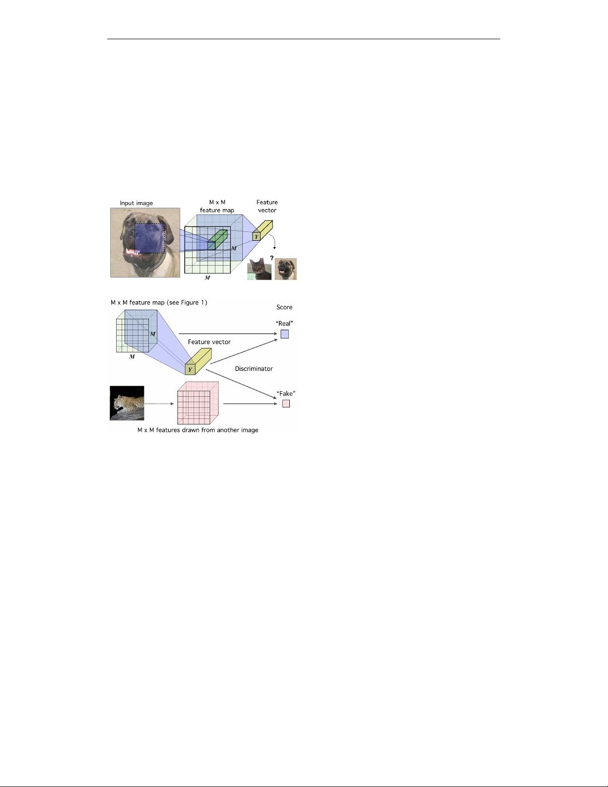
1 INTRODUCTION
One core objective of deep learning is to discover useful representations, and the simple idea explored
here is to train a representation-learning function, i.e. an encoder, to maximize the mutual information
(MI) between its inputs and outputs. MI is notoriously difficult to compute, particularly in continuous
and high-dimensional settings. Fortunately, recent advances enable effective computation of MI
between high dimensional input/output pairs of deep neural networks (Belghazi et al., 2018). We
leverage MI estimation for representation learning and show that, depending on the downstream
task, maximizing MI between the complete input and the encoder output (i.e., global MI) is often
insufficient for learning useful representations. Rather, structure matters: maximizing the average
MI between the representation and local regions of the input (e.g. patches rather than the complete
image) can greatly improve the representation’s quality for, e.g., classification tasks, while global MI
plays a stronger role in the ability to reconstruct the full input given the representation.
Usefulness of a representation is not just a matter of information content: representational char-
acteristics like independence also play an important role (Gretton et al., 2012; Hyv
¨
arinen & Oja,
2000; Hinton, 2002; Schmidhuber, 1992; Bengio et al., 2013; Thomas et al., 2017). We combine MI
maximization with prior matching in a manner similar to adversarial autoencoders (AAE, Makhzani
et al., 2015) to constrain representations according to desired statistical properties. This approach is
closely related to the infomax optimization principle (Linsker, 1988; Bell & Sejnowski, 1995), so we
call our method Deep InfoMax (DIM). Our main contributions are the following:
•
We formalize Deep InfoMax (DIM), which simultaneously estimates and maximizes the
mutual information between input data and learned high-level representations.
•
Our mutual information maximization procedure can prioritize global or local information,
which we show can be used to tune the suitability of learned representations for classification
or reconstruction-style tasks.
•
We use adversarial learning (
`
a la Makhzani et al., 2015) to constrain the representation to
have desired statistical characteristics specific to a prior.
1
Published as a conference paper at ICLR 2019
•
We introduce two new measures of representation quality, one based on Mutual Information
Neural Estimation (MINE, Belghazi et al., 2018) and a neural dependency measure (NDM)
based on the work by Brakel & Bengio (2017), and we use these to bolster our comparison
of DIM to different unsupervised methods.
2 RELATED WORK
There are many popular methods for learning representations. Classic methods, such as independent
component analysis (ICA, Bell & Sejnowski, 1995) and self-organizing maps (Kohonen, 1998),
generally lack the representational capacity of deep neural networks. More recent approaches
include deep volume-preserving maps (Dinh et al., 2014; 2016), deep clustering (Xie et al., 2016;
Chang et al., 2017), noise as targets (NAT, Bojanowski & Joulin, 2017), and self-supervised or
co-learning (Doersch & Zisserman, 2017; Dosovitskiy et al., 2016; Sajjadi et al., 2016).
Generative models are also commonly used for building representations (Vincent et al., 2010; Kingma
et al., 2014; Salimans et al., 2016; Rezende et al., 2016; Donahue et al., 2016), and mutual information
(MI) plays an important role in the quality of the representations they learn. In generative models that
rely on reconstruction (e.g., denoising, variational, and adversarial autoencoders, Vincent et al., 2008;
Rifai et al., 2012; Kingma & Welling, 2013; Makhzani et al., 2015), the reconstruction error can be
related to the MI as follows:
I
e
(X, Y ) = H
e
(X) − H
e
(X|Y ) ≥ H
e
(X) − R
e,d
(X|Y ), (1)
where
X
and
Y
denote the input and output of an encoder which is applied to inputs sampled from
some source distribution.
R
e,d
(X|Y )
denotes the expected reconstruction error of
X
given the codes
Y
.
H
e
(X)
and
H
e
(X|Y )
denote the marginal and conditional entropy of
X
in the distribution formed
by applying the encoder to inputs sampled from the source distribution. Thus, in typical settings,
models with reconstruction-type objectives provide some guarantees on the amount of information
encoded in their intermediate representations. Similar guarantees exist for bi-directional adversarial
models (Dumoulin et al., 2016; Donahue et al., 2016), which adversarially train an encoder / decoder
to match their respective joint distributions or to minimize the reconstruction error (Chen et al., 2016).
Mutual-information estimation
Methods based on mutual information have a long history in
unsupervised feature learning. The infomax principle (Linsker, 1988; Bell & Sejnowski, 1995),
as prescribed for neural networks, advocates maximizing MI between the input and output. This
is the basis of numerous ICA algorithms, which can be nonlinear (Hyv
¨
arinen & Pajunen, 1999;
Almeida, 2003) but are often hard to adapt for use with deep networks. Mutual Information Neural
Estimation (MINE, Belghazi et al., 2018) learns an estimate of the MI of continuous variables, is
strongly consistent, and can be used to learn better implicit bi-directional generative models. Deep
InfoMax (DIM) follows MINE in this regard, though we find that the generator is unnecessary.
We also find it unnecessary to use the exact KL-based formulation of MI. For example, a simple
alternative based on the Jensen-Shannon divergence (JSD) is more stable and provides better results.
We will show that DIM can work with various MI estimators. Most significantly, DIM can leverage
local structure in the input to improve the suitability of representations for classification.
Leveraging known structure in the input when designing objectives based on MI maximization is
nothing new (Becker, 1992; 1996; Wiskott & Sejnowski, 2002), and some very recent works also
follow this intuition. It has been shown in the case of discrete MI that data augmentations and other
transformations can be used to avoid degenerate solutions (Hu et al., 2017). Unsupervised clustering
and segmentation is attainable by maximizing the MI between images associated by transforms or
spatial proximity (Ji et al., 2018). Our work investigates the suitability of representations learned
across two different MI objectives that focus on local or global structure, a flexibility we believe is
necessary for training representations intended for different applications.
Proposed independently of DIM, Contrastive Predictive Coding (CPC, Oord et al., 2018) is a MI-
based approach that, like DIM, maximizes MI between global and local representation pairs. CPC
shares some motivations and computations with DIM, but there are important ways in which CPC and
DIM differ. CPC processes local features sequentially to build partial “summary features”, which are
used to make predictions about specific local features in the “future” of each summary feature. This
equates to ordered autoregression over the local features, and requires training separate estimators
2
Published as a conference paper at ICLR 2019
for each temporal offset at which one would like to predict the future. In contrast, the basic version
of DIM uses a single summary feature that is a function of all local features, and this “global” feature
predicts all local features simultaneously in a single step using a single estimator. Note that, when
using occlusions during training (see Section 4.3 for details), DIM performs both “self” predictions
and orderless autoregression.
3 DEEP INFOMAX
Figure 1:
The base encoder model in the
context of image data.
An image (in this
case) is encoded using a convnet until reach-
ing a feature map of
M × M
feature vec-
tors corresponding to
M × M
input patches.
These vectors are summarized into a single
feature vector,
Y
. Our goal is to train this net-
work such that useful information about the
input is easily extracted from the high-level
features.
Figure 2:
Deep InfoMax (DIM) with a
global MI(X; Y ) objective.
Here, we pass
both the high-level feature vector,
Y
, and the
lower-level
M ×M
feature map (see Figure 1)
through a discriminator to get the score. Fake
samples are drawn by combining the same
feature vector with a
M × M
feature map
from another image.
Here we outline the general setting of training an encoder to maximize mutual information between
its input and output. Let
X
and
Y
be the domain and range of a continuous and (almost everywhere)
differentiable parametric function,
E
ψ
: X → Y
with parameters
ψ
(e.g., a neural network). These
parameters define a family of encoders,
E
Φ
= {E
ψ
}
ψ∈Ψ
over
Ψ
. Assume that we are given a set of
training examples on an input space,
X
:
X := {x
(i)
∈ X }
N
i=1
, with empirical probability distribution
P
. We define
U
ψ,P
to be the marginal distribution induced by pushing samples from
P
through
E
ψ
.
I.e.,
U
ψ,P
is the distribution over encodings
y ∈ Y
produced by sampling observations
x ∼ X
and
then sampling y ∼ E
ψ
(x).
An example encoder for image data is given in Figure 1, which will be used in the following sections,
but this approach can easily be adapted for temporal data. Similar to the infomax optimization
principle (Linsker, 1988), we assert our encoder should be trained according to the following criteria:
• Mutual information maximization:
Find the set of parameters,
ψ
, such that the mutual
information,
I(X; E
ψ
(X))
, is maximized. Depending on the end-goal, this maximization
can be done over the complete input, X, or some structured or “local” subset.
• Statistical constraints:
Depending on the end-goal for the representation, the marginal
U
ψ,P
should match a prior distribution,
V
. Roughly speaking, this can be used to encourage
the output of the encoder to have desired characteristics (e.g., independence).
The formulation of these two objectives covered below we call Deep InfoMax (DIM).
3.1 MUTUAL INFORMATION ESTIMATION AND MAXIMIZATION
Our basic mutual information maximization framework is presented in Figure 2. The approach
follows Mutual Information Neural Estimation (MINE, Belghazi et al., 2018), which estimates mutual
information by training a classifier to distinguish between samples coming from the joint,
J
, and the
3
Published as a conference paper at ICLR 2019
Figure 3:
Maximizing mutual information
between local features and global features.
First we encode the image to a feature map
that reflects some structural aspect of the data,
e.g. spatial locality, and we further summarize
this feature map into a global feature vector
(see Figure 1). We then concatenate this fea-
ture vector with the lower-level feature map
at every location. A score is produced for
each local-global pair through an additional
function (see the Appendix A.2 for details).
product of marginals,
M
, of random variables
X
and
Y
. MINE uses a lower-bound to the MI based
on the Donsker-Varadhan representation (DV, Donsker & Varadhan, 1983) of the KL-divergence,
I(X; Y ) := D
KL
(J||M) ≥
b
I
(DV )
ω
(X; Y ) := E
J
[T
ω
(x, y)] − log E
M
[e
T
ω
(x,y)
], (2)
where
T
ω
: X × Y → R
is a discriminator function modeled by a neural network with parameters
ω
.
At a high level, we optimize E
ψ
by simultaneously estimating and maximizing I(X, E
ψ
(X)),
(ˆω,
ˆ
ψ)
G
= arg max
ω,ψ
b
I
ω
(X; E
ψ
(X)), (3)
where the subscript G denotes “global” for reasons that will be clear later. However, there are some
important differences that distinguish our approach from MINE. First, because the encoder and
mutual information estimator are optimizing the same objective and require similar computations, we
share layers between these functions, so that
E
ψ
= f
ψ
◦ C
ψ
and
T
ψ,ω
= D
ω
◦ g ◦ (C
ψ
, E
ψ
)
,
1
where
g is a function that combines the encoder output with the lower layer.
Second, as we are primarily interested in maximizing MI, and not concerned with its precise value,
we can rely on non-KL divergences which may offer favourable trade-offs. For example, one could
define a Jensen-Shannon MI estimator (following the formulation of Nowozin et al., 2016),
b
I
(JSD)
ω,ψ
(X; E
ψ
(X)) := E
P
[−sp(−T
ψ,ω
(x, E
ψ
(x)))] − E
P×
˜
P
[sp(T
ψ,ω
(x
0
, E
ψ
(x)))], (4)
where
x
is an input sample,
x
0
is an input sampled from
˜
P = P
, and
sp(z) = log(1+e
z
)
is the softplus
function. A similar estimator appeared in Brakel & Bengio (2017) in the context of minimizing the
total correlation, and it amounts to the familiar binary cross-entropy. This is well-understood in terms
of neural network optimization and we find works better in practice (e.g., is more stable) than the
DV-based objective (e.g., see App. A.3). Intuitively, the Jensen-Shannon-based estimator should
behave similarly to the DV-based estimator in Eq. 2, since both act like classifiers whose objectives
maximize the expected
log
-ratio of the joint over the product of marginals. We show in App. A.1 the
relationship between the JSD estimator and the formal definition of mutual information.
Noise-Contrastive Estimation (NCE, Gutmann & Hyv
¨
arinen, 2010; 2012) was first used as a bound
on MI in Oord et al. (and called “infoNCE”, 2018), and this loss can also be used with DIM by
maximizing:
b
I
(infoNCE)
ω,ψ
(X; E
ψ
(X)) := E
P
"
T
ψ,ω
(x, E
ψ
(x)) − E
˜
P
"
log
X
x
0
e
T
ψ,ω
(x
0
,E
ψ
(x))
##
. (5)
For DIM, a key difference between the DV, JSD, and infoNCE formulations is whether an expectation
over
P/
˜
P
appears inside or outside of a
log
. In fact, the JSD-based objective mirrors the original
NCE formulation in Gutmann & Hyv
¨
arinen (2010), which phrased unnormalized density estimation
as binary classification between the data distribution and a noise distribution. DIM sets the noise
distribution to the product of marginals over
X/Y
, and the data distribution to the true joint. The
infoNCE formulation in Eq. 5 follows a softmax-based version of NCE (Jozefowicz et al., 2016),
similar to ones used in the language modeling community (Mnih & Kavukcuoglu, 2013; Mikolov et al.,
1
Here we slightly abuse the notation and use ψ for both parts of E
ψ
.
4
Published as a conference paper at ICLR 2019
2013), and which has strong connections to the binary cross-entropy in the context of noise-contrastive
learning (Ma & Collins, 2018). In practice, implementations of these estimators appear quite similar
and can reuse most of the same code. We investigate JSD and infoNCE in our experiments, and
find that using infoNCE often outperforms JSD on downstream tasks, though this effect diminishes
with more challenging data. However, as we show in the App. (A.3), infoNCE and DV require a
large number of negative samples (samples from
˜
P
) to be competitive. We generate negative samples
using all combinations of global and local features at all locations of the relevant feature map, across
all images in a batch. For a batch of size
B
, that gives
O(B × M
2
)
negative samples per positive
example, which quickly becomes cumbersome with increasing batch size. We found that DIM with
the JSD loss is insensitive to the number of negative samples, and in fact outperforms infoNCE as the
number of negative samples becomes smaller.
3.2 LOCAL MUTUAL INFORMATION MAXIMIZATION
The objective in Eq. 3 can be used to maximize MI between input and output, but ultimately this
may be undesirable depending on the task. For example, trivial pixel-level noise is useless for image
classification, so a representation may not benefit from encoding this information (e.g., in zero-shot
learning, transfer learning, etc.). In order to obtain a representation more suitable for classification,
we can instead maximize the average MI between the high-level representation and local patches of
the image. Because the same representation is encouraged to have high MI with all the patches, this
favours encoding aspects of the data that are shared across patches.
Suppose the feature vector is of limited capacity (number of units and range) and assume the encoder
does not support infinite output configurations. For maximizing the MI between the whole input and
the representation, the encoder can pick and choose what type of information in the input is passed
through the encoder, such as noise specific to local patches or pixels. However, if the encoder passes
information specific to only some parts of the input, this does not increase the MI with any of the
other patches that do not contain said noise. This encourages the encoder to prefer information that is
shared across the input, and this hypothesis is supported in our experiments below.
Our local DIM framework is presented in Figure 3. First we encode the input to a feature map,
C
ψ
(x) := {C
(i)
ψ
}
M×M
i=1
that reflects useful structure in the data (e.g., spatial locality), indexed in this
case by
i
. Next, we summarize this local feature map into a global feature,
E
ψ
(x) = f
ψ
◦ C
ψ
(x)
.
We then define our MI estimator on global/local pairs, maximizing the average estimated MI:
(ˆω,
ˆ
ψ)
L
= arg max
ω,ψ
1
M
2
M
2
X
i=1
b
I
ω,ψ
(C
(i)
ψ
(X); E
ψ
(X)). (6)
We found success optimizing this “local” objective with multiple easy-to-implement architectures,
and further implementation details are provided in the App. (A.2).
3.3 MATCHING REPRESENTATIONS TO A PRIOR DISTRIBUTION
Absolute magnitude of information is only one desirable property of a representation; depending on
the application, good representations can be compact (Gretton et al., 2012), independent (Hyv
¨
arinen
& Oja, 2000; Hinton, 2002; Dinh et al., 2014; Brakel & Bengio, 2017), disentangled (Schmidhuber,
1992; Rifai et al., 2012; Bengio et al., 2013; Chen et al., 2018; Gonzalez-Garcia et al., 2018), or
independently controllable (Thomas et al., 2017). DIM imposes statistical constraints onto learned
representations by implicitly training the encoder so that the push-forward distribution,
U
ψ,P
, matches
a prior,
V
. This is done (see Figure 7 in the App. A.2) by training a discriminator,
D
φ
: Y → R
, to
estimate the divergence, D(V||U
ψ,P
), then training the encoder to minimize this estimate:
(ˆω,
ˆ
ψ)
P
= arg min
ψ
arg max
φ
b
D
φ
(V||U
ψ,P
) = E
V
[log D
φ
(y)] + E
P
[log(1 − D
φ
(E
ψ
(x)))]. (7)
This approach is similar to what is done in adversarial autoencoders (AAE, Makhzani et al., 2015),
but without a generator. It is also similar to noise as targets (Bojanowski & Joulin, 2017), but trains
the encoder to match the noise implicitly rather than using a priori noise samples as targets.
5
剩余23页未读,继续阅读
实在想不出来了
- 粉丝: 23
- 资源: 318
上传资源 快速赚钱
- 我的内容管理 展开
- 我的资源 快来上传第一个资源
- 我的收益 登录查看自己的收益
- 我的积分 登录查看自己的积分
- 我的C币 登录后查看C币余额
- 我的收藏
- 我的下载
- 下载帮助
安全验证
文档复制为VIP权益,开通VIP直接复制
信息提交成功
评论0