论文 波束赋形 波束赋形 波束赋形
需积分: 5 89 浏览量
2022-02-11
15:55:43
上传
评论
收藏 2.4MB PDF 举报

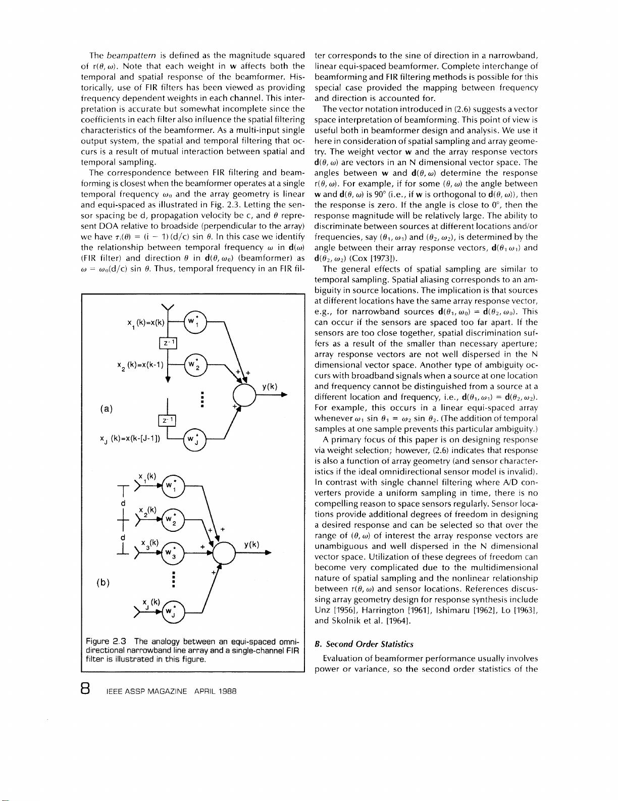
Beamforming:
A
Versatile
Approach to Spatial Filtering
Barry
D.
Van
A
beamformer
is
a processor used in conjunction with an
array of sensors to provide a versatile form of spatial filtering.
The sensor array collects spatial samples of propagating wave
fields, which are processed by the beamformer. The objective
is
to estimate the signal arriving from a desired direction in
the presence of noise and interfering signals.
A
beamformer
performs spatial filtering to separate signals that have over-
lapping frequency content but originate from different spatial
locations. This paper provides an overview of beamforming
from a signal processing perspective, with an emphasis on re-
cent research. Data independent, statistically optimum, adap-
tive, and partially adaptive beamforming are discussed.
1.
INTRODUCTION
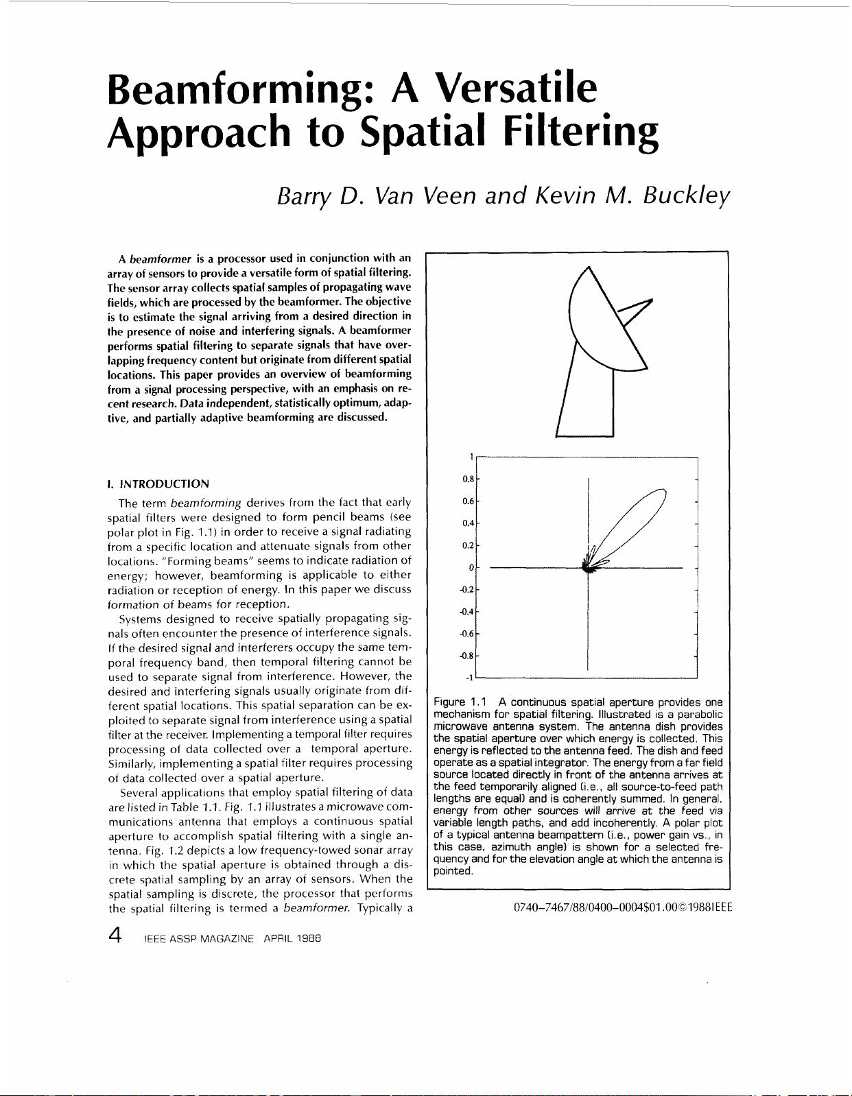
The term beamforming derives from the fact that early
spatial filters were designed to form pencil beams (see
polar plot in Fig.
1
.I)
in order to receive a signal radiating
from
a
specific location and attenuate signals from other
locations. ”Forming beams” seems to indicate radiation of
energy; however, beamforming
is
applicable to either
radiation or reception of energy. In this paper we discuss
formation of beams for reception.
Systems designed to receive spatially propagating sig-
nals often encounter the presence of interference signals.
If the desired signal and interferers occupy the same tem-
poral frequency band, then temporal filtering cannot be
used to separate signal from interference. However, the
desired and interfering signals usually originate from dif-
ferent spatial locations. This spatial separation can be ex-
ploited to separate signal from interference using
a
spatial
filter at the receiver. Implementing
a
temporal filter requires
processing of data collected over
a
temporal aperture.
Similarly, implementing
a
spatial filter requires processing
of data collected over
a
spatial aperture.
Several applications that employ spatial filtering of data
are listed in Table
1
.1.
Fig.
1
.I
illustrates
a
microwave com-
munications antenna that employs
a
continuous spatial
aperture to accomplish spatial filtering with a single an-
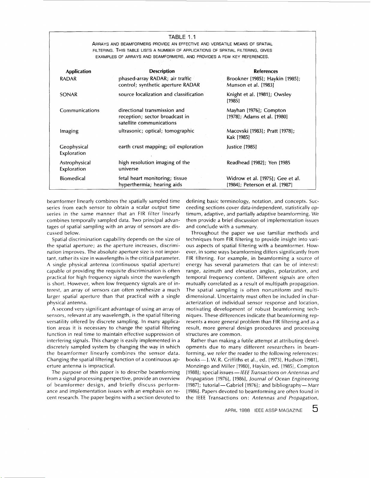
tenna. Fig.
1.2
depicts a low frequency-towed sonar array
in which the spatial aperture
is
obtained through
a
dis-
crete spatial sampling by an array
of
sensors. When the
spatial sampling
is
discrete, the processor that performs
the spatial filtering
is
termed
a
beamformer. Typically
a
4
IEEE
ASSP MAGAZINE APRIL
1988
Veen and Kevin
M.
Buckley
’igure
1
.I
A
continuous spatial aperture provides one
nechanism for spatial filtering. Illustrated is a parabolic
nicrowave antenna system. The antenna dish provides
;he spatial aperture over which energy is collected. This
3nergy
is
reflected to the antenna feed. The dish and feed
iperate as a spatial integrator. The energy from a far field
source located directly in front
of
the antenna arrives at
;he feed temporarily aligned [i.e., all source-to-feed path
engths are equal1 and
is
coherently summed. In general,
?nergy from other sources will arrive at the feed via
iariable length paths, and add incoherently.
A
polar plot
if
a typical antenna beampattern (i.e., power gain
vs.,
in
;his case, azimuth angle1
is
shown for a selected fre-
iuency and for the elevation angle at which the antenna
is
minted.
0740-746718810400-0004$01
.OOGI9881
EEE
剩余20页未读,继续阅读


qq_45884246
- 粉丝: 0
- 资源: 9


最新资源
- 基于matlab实现用有限元法计算电磁场的Matlab工具 .rar
- 基于matlab实现有限元算法 计算电磁场问题 边界条件包括第一类边界和第二类边界.rar
- 基于matlab实现用于计算不同车重下的电动汽车动力性和经济性.rar
- 基于matlab实现遗传算法求解多车场车辆路径问题 有多组算例可以用.rar
- 浏览器.apk
- 基于matlab实现是一个matlab中的power system 中搭建的一个模型
- 基于JSP毕业设计-教学管理系统(源代码+论文).zip
- 基于JSP毕业设计-家政管理系统-毕业设计.zip
- 基于Python实现淘宝商品评论采集(含逆向)源代码
- 基于matlab实现多目标进化算法NSGAⅡ&Matlab讲解.rar
资源上传下载、课程学习等过程中有任何疑问或建议,欢迎提出宝贵意见哦~我们会及时处理!
点击此处反馈


评论0