2/14/2018 DIC Algorithms
http://www.ncorr.com/index.php/dic-algorithms#1_1 1/22
DIC Algorithms
Table of Contents
1 - DIC Analysis
1.1 - The general problem
2 - Computational Implementation
2.1 - Correlation criteria
3 - Nonlinear Optimization
3.1 - The initial guess
3.2 - Gauss-Newton nonlinear iterative least squares method
3.3 - Forward additive method
3.4 - Inverse compositional method
3.5 - Computation of the gradient and hessian for the IC-GN method
3.6 - Biquintic B-spline background theory
3.7 - Biquintic B-spline implementation
3.8 - Inverse compositional method summary
4 - Obtaining Full Field Displacements
5 - Obtaining Full Field Strains
6 - Concluding Remarks
7 - Citations
1 - DIC Analysis
The intent of this write up is to provide an explanation of the mathematical framework and modern algorithms used in Ncorr, and in 2D-DIC in general. If the reader is already
familiar with DIC and would simply like to use Ncorr or experiment with it first, it is available for download in the downloads section of this website.
1.1 - The general problem
Home
Downloads
C++ Port
Publications
Applications
DIC Algorithms
Data Collection
Contact/About

2/14/2018 DIC Algorithms
http://www.ncorr.com/index.php/dic-algorithms#1_1 2/22
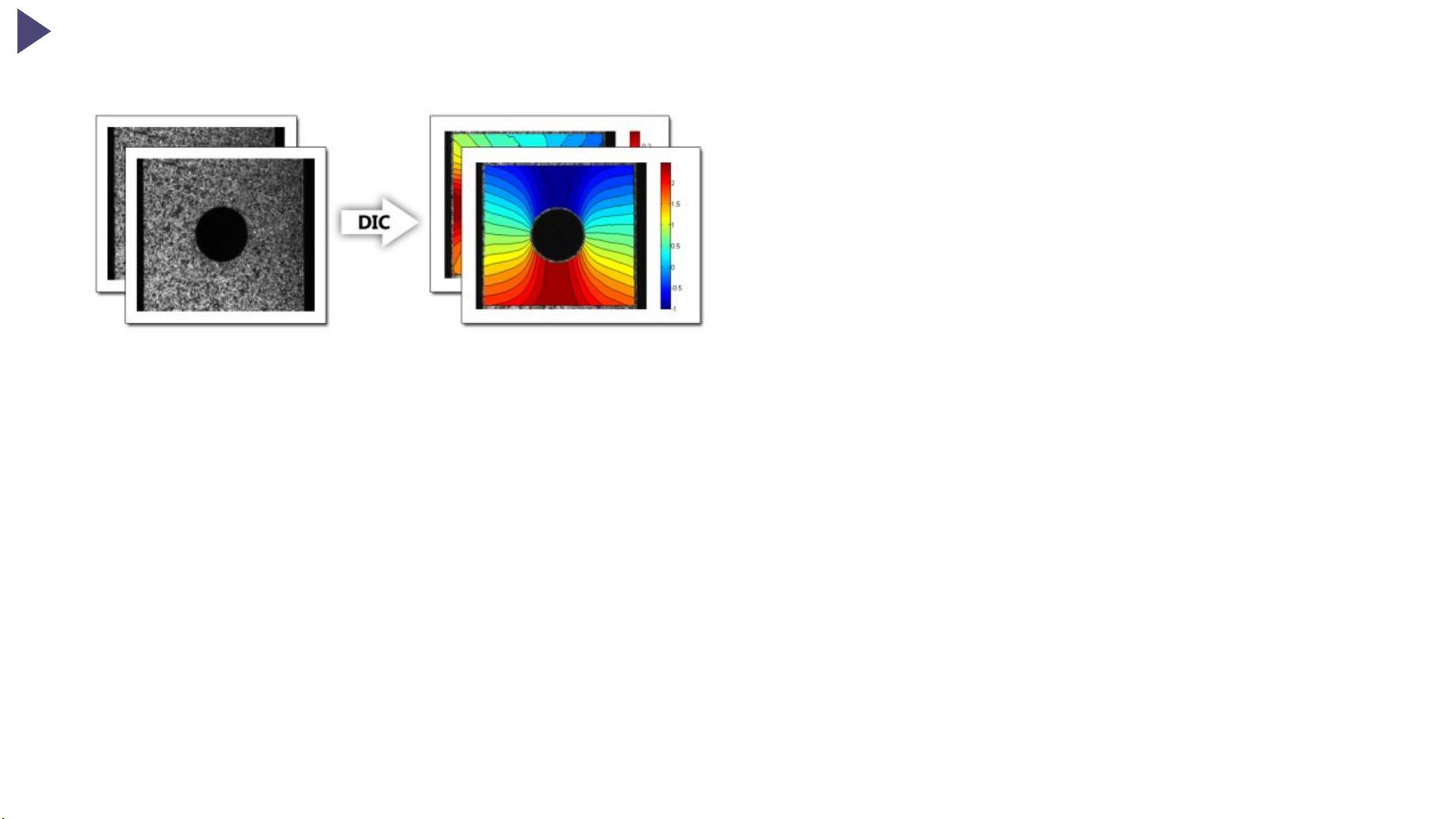
The overall goal of DIC is to obtain displacement and strain fields within a region of interest (ROI) for a material sample undergoing deformation. DIC uses image processing
techniques in an attempt to solve this problem. Basically, images of a sample are taken as it deforms; these images are used as inputs to a DIC program. The idea is to somehow
obtain a one-to-one correspondence between material points in the reference (initial undeformed picture) and current (subsequent deformed pictures) configurations. DIC does
this by taking small subsections of the reference image, called subsets, and determining their respective locations in the current configuration. For each subset, we obtain
displacement and strain information through the transformation used to match the location of the subset in the current configuration. Many subsets are picked in the reference
configuration, often with a spacing parameter to reduce computational cost (also note that subsets typically overlap as well). The end result is a grid containing displacement and
strain information with respect to the reference configuration, also referred to as Lagrangian displacements/strains. The displacement/strain fields can then either be reduced or
interpolated to form a "continuous" displacement/strain field. These ideas will be made more precise in the following sections.
2 - Computational Implementation
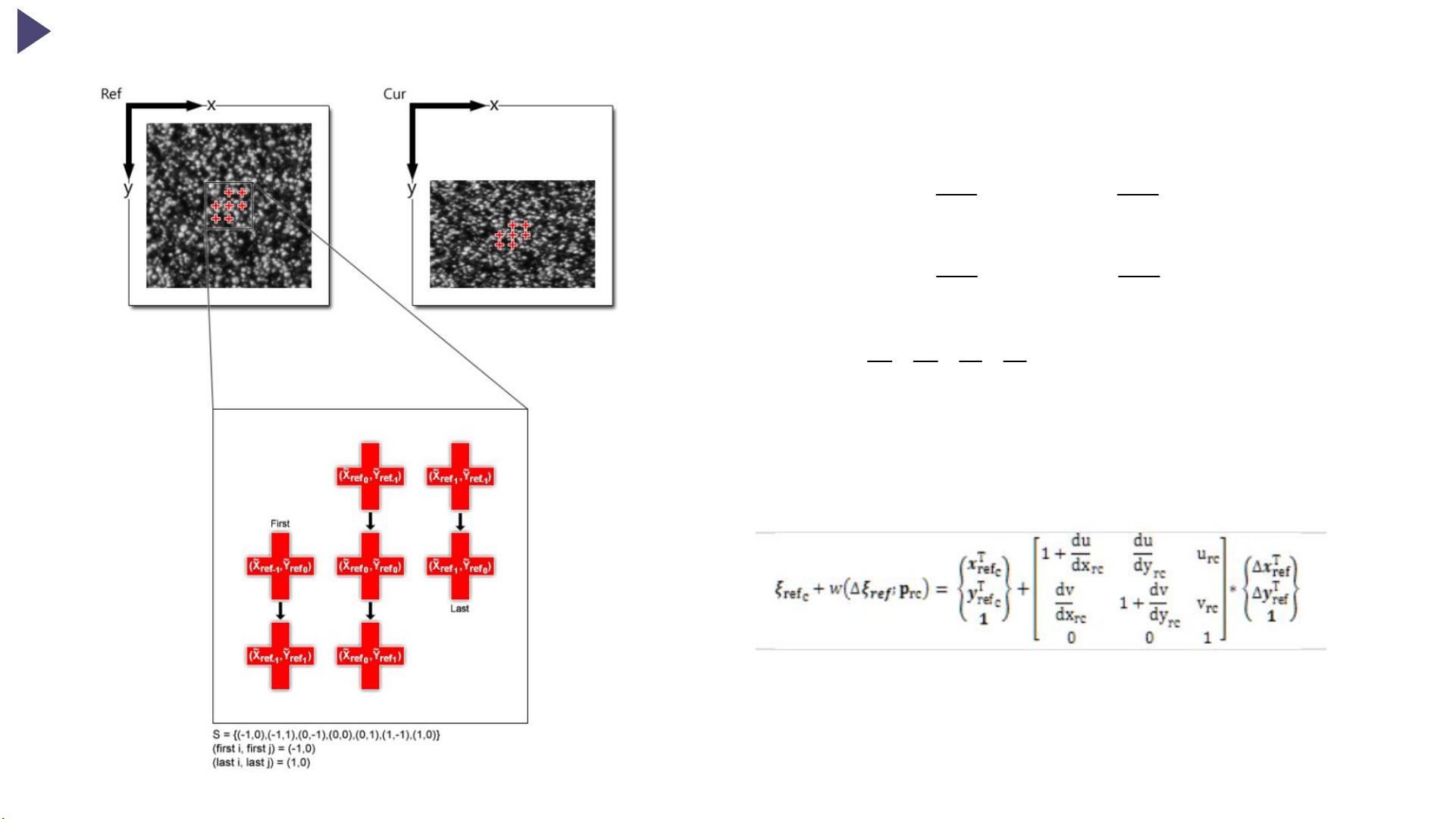
To be more specific, subsets are essentially a group of coordinate points; the idea of subsets in the reference and current image is shown in fig.1.
Fig.1. The subset's coordinates are shown as red crosses. The notation at the bottom is used throughout the rest of this document. The subset does not need to be square, as
shown above; the shape can be arbitrary as long as it contains a center point.
The transformation of initial reference subset points to the current configuration is typically constrained to a linear, first order transformation (although second order
transformations can also be used if very large strains are anticipated[1]) as shown below:
Eq.1

2/14/2018 DIC Algorithms
http://www.ncorr.com/index.php/dic-algorithms#1_1 3/22
Eq.2
Where and are the x and y coordinates of an initial reference subset point, and are the x and y coordinates of the center of the initial reference subset,
and are the x and y coordinates of a final current subset point, (i,j) are indices used for the relative location of the subset points with respect to the center of the subset, as
well as for correspondences between subset points in the current and reference configuration, and S is a set which contains all of the subset points (an example is given in fig.1).
The subscript "rc" used in eq.1 is meant to signify that the transformation is from the reference to the current coordinate system. Furthermore, is the general
form of the deformation vector, p, as defined in eq.2 (its effect on subsets is shown in fig.2). Lastly, eq.1 can also be written in matrix form as shown below:
Eq.3
Where is an augmented vector containing the x and y coordinates of subset points, Δx and Δy are the distance between a subset point and the center of the subset,and "w" is a
function called a warp. For computational purposes, we also allow the reference subset to deform within the reference configuration, as shown below:
Eq.4
Where and are x and y coordinates of a final reference subset point. The "rr" subscript in eq.4 is meant to signify that the transformation is from the reference coordinate
system to the reference coordinate system.
For our purposes, we want to find the optimal p
rc
, when p
rr
= 0, such that the coordinates at and best match the coordinates at and , respectively. I denote this
p
rc
value . For now, it may seem nonsensical to even use eq.4 and just restrict the reference subset coordinates such that they are undeformable. But, one of the methods we
will eventually use to find (the inverse compositional method) requires the reference subset coordinates to be deformable, so I introduced this notation now to make the
subsequent derivation smoother.
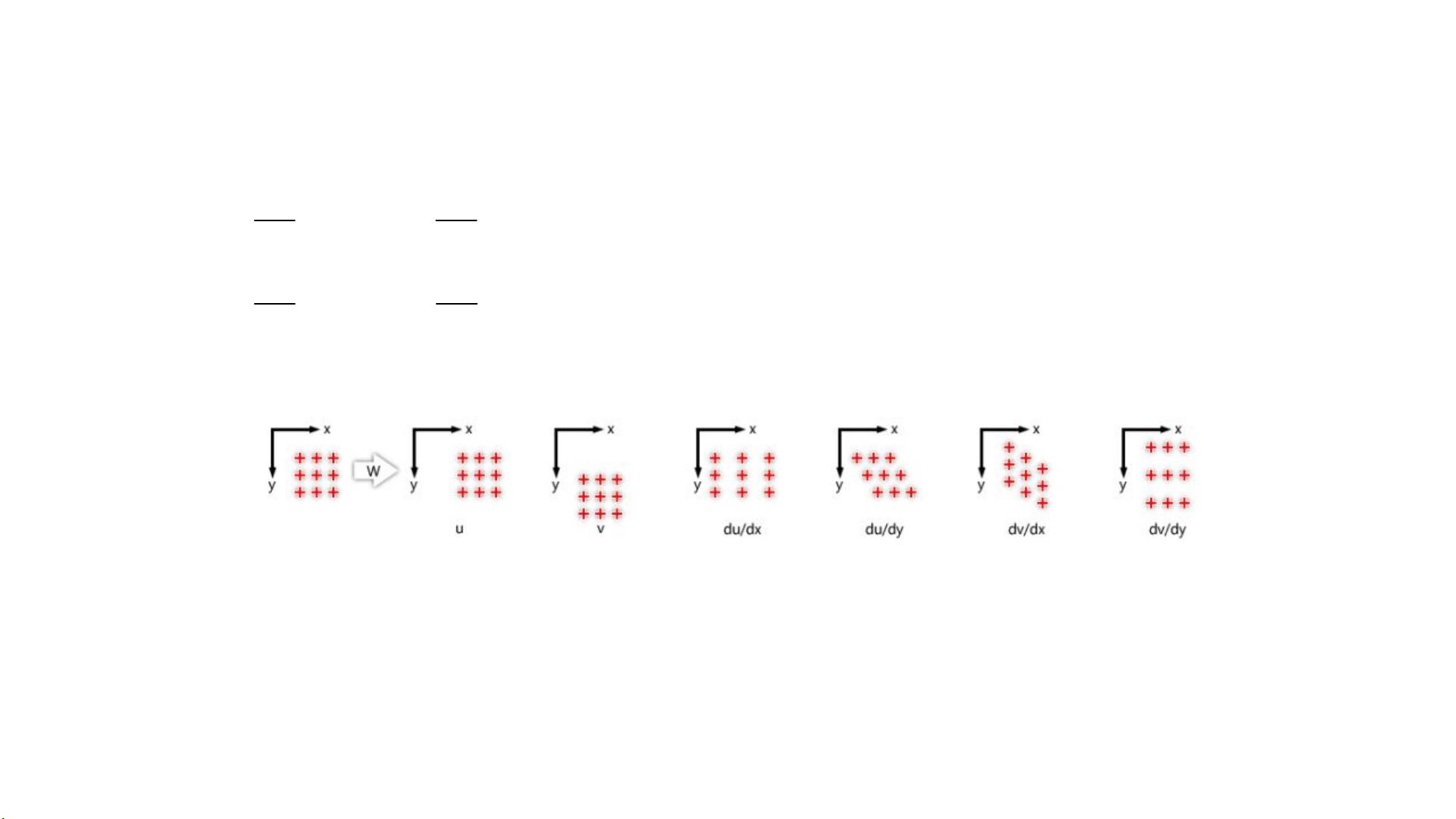
Fig.2. The above figure shows linear transformations for subset coordinates. Any linear combination of the 6 parameters shown above can be used to deform subset
coordinates through a warp function, w.
2.1 - Correlation criteria
The next step is to establish a metric for similarity between the final reference subset and final current subset. This is carried out by comparing grayscale values at the final
reference subset points with gray scale values at the final current subset points. The following two metrics are the most commonly used in DIC:
Eq.5
Eq.6

2/14/2018 DIC Algorithms
http://www.ncorr.com/index.php/dic-algorithms#1_1 4/22
Where f and g are the reference and current image functions, respectively, and return a grayscale value corresponding to the specified (x,y) point. f
m
and g
m
are the mean
grayscale values of the final reference and current subset, respectively, as defined by:
Eq.7
Eq.8
Where n(S) is the number of elements in S.
Eq.5 is the normalized cross correlation criterion and indicates a good match when C
CC
is close to 1. Eq.6 is the normalized least squares criterion and indicates a good match
when C
LS
is close to 0. Subtraction of the mean component (f
m
and g
m
) in eq.5-6 allow for the criteria to be invariant to shifts in grayscale values, while division by the quantity in
the denominator allow for invariance with respect to scaled grayscale values; the end result is correlation criteria which are invariant to affine shifts in grayscale values. In
actuality, these correlation criteria are directly related [2], but each respective correlation criterion is easier to calculate in certain situations which is why both are listed. A simple
example of how both are used is given in fig.3.
Fig.3. The above figure demonstrates the effectiveness of the two correlation criteria. The grayscale values on the left are compared with the two on the right. The correlation
criteria show that the top right gray scale values match the set on the left (C
CC
is close to 1 and C
LS
is close to 0), which is obvious through visual inspection.
The general steps for the utilization of these correlation criteria are outlined below:
1. Form an initial subset in the reference configuration, typically at integer pixel locations. Apply a warp, with p
rr
, to the initial reference subset and sample f, the reference
gray scale values, at these points and store these values in an array
2. Apply a warp, with p
rc
, to the initial reference subset to bring it to the current configuration. Sample g, the current gray scale values, at these points and store them in an
equivalent sized array as in step 1 (note that the storing of these points is essentially an inverse transformation and allows for a direct correspondence/comparison between
grayscale values in the reference and current configuration).
3. Now you can compare these two arrays using either of the two correlation criteria in eqs.5-6. This process is outlined in the figure below:

2/14/2018 DIC Algorithms
http://www.ncorr.com/index.php/dic-algorithms#1_1 5/22
Fig.4. This figure is a graphical example of the steps outlined above. The green subset in the reference image is the initial reference subset. The red subsets mark the final
subset locations in the reference and current configuration.
Note that if p
rr
and p
rc
are found so that the final subsets match well, and p
rr
is small in translational magnitude, then can be approximated by taking p
rc
and composing it with
the inverse of p
rr
. Imagine this as a direct transformation from the final reference subset to the final current subset. This idea is important for an understanding of the inverse
compositional algorithm which is discussed later.
Anyway, the next step of the analysis is how to establish a method to find in an automated way. The main implementation in DIC is to use an iterative nonlinear least squares
optimization scheme which minimizes eq.6 (note that eq.6 is strictly positive and a smaller number indicates a better match).
3 - Nonlinear Optimization
The nonlinear optimization section is broken into three main parts: 1) providing an initial guess, 2) the Gauss-Newton (GN) iterative optimization scheme and 3) interpolation. An
initial guess is required because iterative optimization schemes converge to a local maximum/minimum; thus, an initial guess near the global maximum/minimum is required. In
the GN iterative optimization scheme section, two different schemes are discussed: the forward additive Gauss-Newton method (FA-GN), and the inverse compositional Gauss-
Newton method (IC-GN). The FA-GN method is discussed first because this is a commonly utilized algorithm in DIC (and in optimization in general) . On the other hand, the IC-
GN method is a special case of nonlinear optimization (commonly utilized in image alignment algorithms) which is faster than the standard FA-GN method and was recently
applied to DIC [3]. Lastly, interpolation is discussed because grayscale values and gradients at subpixel locations are required to compute quantities used in the FA-GN and IC-
GN methods.
The general flow of a nonlinear optimization scheme is shown below:


