K-DBSCAN:IdentifyingSpatialClustersWithDifferingDensityLevels资源-CSDN文库

机器学习

DBSCAN

需积分: 10 174 浏览量 2018-10-09 17:12:35 上传评论 1 收藏 703KB PDF 举报

资源推荐

资源详情

资源评论

K-DBSCAN: Identifying Spatial Clusters With

Differing Density Levels

Madhuri Debnath

Department of Computer Science

and Engineering

University of Texas at Arlington

Arlington, Texas

Email: madhuri.debnath@mavs.uta.edu

Praveen Kumar Tripathi

Department of Computer Science

and Engineering

University of Texas at Arlington

Arlington, Texas

Email: p raveen.tripathi@mavs.uta.edu

Ramez Elmasri

Department of Computer Science

and Engineering

University of Texas at Arlington

Arlington, Texas

Email: elmasri@cse.uta.edu

Abstract—Spatial clustering is a very important tool in the

analysis of spatial data. In this paper, we propose a novel

density based spatial clustering algorithm called K-DBSCAN with

the main focus of identifying clusters of points with similar

spatial density. This contrasts with many other approaches,

whose main focus is spatial contiguity. The strength of K-

DBSCAN lies in ﬁnding arbitrary shaped clusters in variable

density regions. Moreover, it can also discover clusters with

overlapping spatial regions, but differing density levels. The goal

is to differentiate the most d ense regions from lower density

regions, with spatial contiguity a s the secondary goal. The original

DBSCAN fails to discover the clusters with variable density and

overlapping regions. OPTICS and Shared Nearest Neighbour

(SNN) algorithms have the capabilities of clustering variable

density datasets but they have their own limitations. Both fail to

detect overlapping clusters. Also, while handling varying density,

both of the algorithms merge points from different density levels.

K-DBSCAN has two phases: ﬁrst, it d ivides all data objects

into different density levels to identify the different natural

densities present in the dataset; then it extracts the clusters using

a modiﬁed version of DBSCAN. Experimental results on both

synthetic data and a real-world spatial dataset demonstrate the

effectiveness of our clustering algorithm.

I. INTRODUCTION

Clustering is the process of grouping a set of objects into

classes or clusters so that the similarity between the objects

within the same cluster is maximized. For researchers who

work with geographical and other types of spatial data, data

mining has offered many useful and promising tools for data

analysis. Spatial clustering is one of these tools [1].

Spatial Clu stering has a wide range of applications. Some

of them include crime hot-spot analysis, identiﬁcation of sim-

ilar land usage, earthquake analysis, agricultural environment

analysis and merging of regions with similar weather patterns.

Spatial databases have some unique challenges. So, in

order to choose a clustering algorithm that is suitable for a

particular spatial application, some important issues need to

be considered [2].

• Clustering algorithms should identify irregular shapes.

Partitioning algorithms like K-means [3] or K-medoids

[4] can discover clusters with spherical shapes and

similar size. Density-based clustering alg orithms like

DBSCAN [5] are more suitable to ﬁnd arbitrary

shaped clusters.

• The algorithms should not be sensitive to the order

of input. That means, clustering results should be

independent of data order. For example, cluster quality

and efﬁciency in K-means [3] depends on the choice

of initial seeds, while cluster results in DBSCAN [5]

do not depend on the data order.

• Algorithms should handle data with outliers. Density-

based algorithms like DBSCAN [5] and OPTICS [6]

can handle noise, while K-means [3] cannot.

• Algorithms should not be too sensitive to user spec-

iﬁed parameter. For example, existing density-based

algorithms like DBSCAN [5], DENCLUE [7] and

OPTICS [6] need a careful choice of threshold for

density, because they may produce very different

results even for slightly different parameter settings.

• Lastly, clustering algorithms should handle spatial data

with varying density. DBSCAN [5] fails to cluster this

kind of data.

Motivated by these challenges, we propose a new density-

based spatial clustering algorithm K-DBSCAN to analyse

spatial data that can handle data with different density levels.

Unlike the DBSCAN [5] algorithm, it does not depend on the

global  parameter to calculate neighbourhood, rather each data

point dynamically generates its own parameter to deﬁne its

neighbourhood. Hence, it has less sensitivity to user speciﬁed

parameter.

Our proposed K-DBSCAN algorithm can be utilized in

several applications. For example, it can be used to ﬁnd spatial

clusters with differing population density levels, even when

these clusters are overlapping. Spatial analysis of regions based

on population has important application in urban planning,

healthcare and economic development. Population density lev-

els of different regions are d ifferent.

The rest of the paper is organized as follows. In Section

2, we review some related works. We describe our proposed

algorithm in Section 3. Section 4 presents experimental results

of our algorithm and compares the quality of the clustering

result with three other well-known algorithms. In Section 5,

we present a practical application of our algorithm with a real-

world spatial dataset. Finally Section 6 concludes the paper.

2015 International Workshop on Data Mining with Industrial Applications

DOI 10.1109/DMIA.2015.14

2015 International Workshop on Data Mining with Industrial Applications

DOI 10.1109/DMIA.2015.14

II. RELATED WORK

Spatial Clustering algorithms can be partitioned into four

general categories: Partitioning, h ierarchical, density-based and

grid-based.

Partitioning algorithms divide the entire dataset into a

number of disjoint groups. Each disjoint group is a cluster.

K-means [3], EM (Expectation Maximization) [8] and K-

medoid [4] are three well-known partitioning based clustering

algorithms. These use an iterative approach and try to group the

data into K clusters, where K is a u ser speciﬁed parameter. The

shortcoming of the algorithms is that they are not suitable for

ﬁnding arbitrary shaped clusters. Further, they are dependent

on the u ser speciﬁed parameter K.

Hierarchical clustering algorithms use a distance matrix

as an input and generates a hierarchical set of clusters. This

hierarchy is generally formed in two ways: bottom-up and top-

down [4]. The top-down approach starts with all the objects in

the same cluster. In each successive iteration a bigger cluster

is split into smaller clusters based on some distance measure,

until each object is in one cluster itself. The clustering level

is chosen between the root (a single large cluster) and the

leaf nodes (a cluster for each individual object). The bottom-

up approach starts with each object as one cluster. It then

successively merges the clusters until all the clusters are

merged together to form a single big cluster. The weakness

of the hierarchical algorithms is that they are computationally

very expensive.

BIRCH [9] and CURE [10] are hierarchical clustering

algorithms. In BIRCH, data objects are compressed into small

sub-clusters, then the clustering algorithm is applied on these

sub-clusters. In CURE, instead of using a single centroid, a

ﬁxed number of well scattered objects are selected to represent

each cluster.

Density-based methods can ﬁlter out the outliers and can

discover arbitrary shaped clusters. DBSCAN [5] is the ﬁrst

proposed density-based clustering algorithm. This algorithm

is based on two parameters:  and MinPts. Density around

each point depends on the number of neighbours within its

 distance. A data point is considered dense if the number

of its neighbours is greater than MinPts. DBSCAN can

ﬁnd clusters of arbitrary shapes, but it cannot handle data

containing clusters of varying densities. Further, the cluster

quality in DBSCAN algorithm depends on the ability of the

user to select a good set of parameters.

OPTICS [6] is another density based clustering algorithm,

proposed to overcome the major weakness of DBSCAN algo-

rithm. This algorithm can handle data with varying density.

This algorithm does not produce clusters explicitly, rather

computes an augmented cluster ordering such that spatially

closest points become neighbours in that order.

The DENCLUE [7] algorithm was proposed to handle high

dimensional data efﬁciently. In this algorithm density of a data

object is determined based on the sum of inﬂuence functions

of the data points around it. DENCLUE also requires a careful

selection o f clusterin g parameters which may signiﬁcantly

inﬂuence the quality of the clusters.

The Shared Nearest Neighbour (SNN) [11] clustering al-

gorithm was proposed to ﬁnd clusters of different densities

in high dimensional data. A similarity measure is based on

the number of shared neighbours between two objects instead

of traditional Euclidean distance. This algorithm needs 3

parameters (k, , MinPt).

Grid-based clustering algorith m divides the data space into

a ﬁnite number of g rid cells forming a grid structure on

which operations are performed to obtain the clusters. Some

examples of grid based methods include STING [12], Wave-

Cluster [13] and CLIQUE [14]. The STING [12] algorithm

calculates statistical information in each grid cells. The Wave-

Cluster [13] algorithm applies wavelet transformation to the

feature base. Input parameters include the number o f g rid

cells for each dimension. This algorithm is applicable for low

dimensional data space. The CLIQUE [14] algorithm adopts a

combination of grid-based and density-based approaches and

this algorithm can detect clusters in high-dimensional space.

III. P

ROPOSED ALGORITHM

In this section, we focus on the basic steps of our proposed

algorithm. We propose K-DBSCAN algorithm, which works in

two phases.

• K Level Density Partitioning: In this phase, we calcu-

late the density of each data point based on its distance

from its nearest neighbouring data points. Then we

partition all the data points into K groups based on

their density value.

• Density Level Clustering: In this phase, we introduce

a modiﬁed version of DBSCAN algorithm that works

on different density levels.

A. K-DBSCAN Phase 1 - K level Density Partitioning

In real world spatial datasets, different data objects may

be located in different density regions. So, it is very difﬁcult

or almost impossible to characterize the cluster structures by

using only one global density parameter [15].

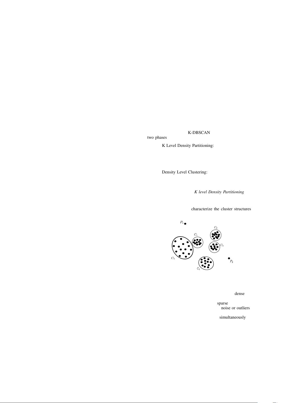
Fig. 1: Points in different density regions

Consider the example from Figure 1. In this example,

points in clusters C

, C

and C

represents very dense neigh-

bourhoods. Points in cluster C

represents a less dense region,

while points in cluster C

represent a sparse neighbourhood.

Point P

and P

should be considered as noise or outliers. As

different data points are located in different density regions, it

is impossible to obtain all the clusters simultaneou sly using

one global density parameter. Because, if we consider the

density estimation for points located in C

, we have to choose

5352

剩余9页未读，继续阅读

评论收藏

内容反馈

Nick_Wang94

粉丝: 37
资源: 3

K-DBSCAN: Identifying Spatial Clusters With Differing Density Le...

最新资源

K-DBSCAN: Identifying Spatial Clusters With Differing Density Le...

Modern Methods And Algorithms Of Quantum Chemistry - Ab Initio Molecular Dynamics Theory 量子化学从头计算方法的现代方法与算法

一个完整的聚类算法,含界面UI和substance.jar

DBSCAN算法 cluster算法

DBSCAN集群

基于DBSCAN聚类算法的研究与实现

DBSCAN算法

DBSCAN（Density-Based Spatial Clustering of Applications with Noise）python实现代码

聚类算法Spatio-temporal-Clustering.zip

DBSCAN.rar_DBSCAN_clustering_dbscan k-means_dbscan matlab_dbscan

由时间空间成对组成的轨迹序列+lstm+自编码器auto-encode+时空密度聚类st-dbscan异常检测源码.zip

ODIC-DBSCAN: 一种新的簇内孤立点分析算法

DBSCAN 算法

DBSCAN聚类算法

DBSCAN算法实现

聚类算法DBSCAN的实现

DBSCAN ST-DBSCAN JavaScript源码

基于MDT重叠覆盖度数据的KNN-DBSCAN参数自适应调优研究.docx

DBSCAN-and-TI-DBSCAN-w.r.t.-cosine-similarity-and-Euclidean-measure:DBSCAN +和TI-DBSCAN + wrt余弦相似度和欧几里得测度

基于PB-DBSCAN的GPS数据去噪.pdf

DBSCAN:Objective-C Implementation of Density-Based Spatial Clustering of Applications with Noise (基于密度的聚类算法)

dbscan(clustering algorithm)

k-cluster样本数据

一种dbscan聚类改进算法

K-means&K-means2&K-means sklearn&DBSCAN-python代码实现-源码.zip

机器学习-python-实验-DBSCAN-BIRCH-对比k-means model & 高斯混合模型

最新资源