DeepResidualLearningforImageRecognition.pdf资源-CSDN文库

论文

10 浏览量 2024-11-19 16:06:22 上传评论收藏 1.34MB PDF 举报

资源推荐

资源详情

资源评论

Deep Residual Learning for Image Recognition

Kaiming He Xiangyu Zhang Shaoqing Ren Jian Sun

Microsoft Research

{kahe, v-xiangz, v-shren, jiansun}@microsoft.com

Abstract

Deeper neural networks are more difﬁcult to train. We

present a residual learning framework to ease the training

of networks that are substantially deeper than those used

previously. We explicitly reformulate the layers as learn-

ing residual functions with reference to the layer inputs, in-

stead of learning unreferenced functions. We provide com-

prehensive empirical evidence showing that these residual

networks are easier to optimize, and can gain accuracy from

considerably increased depth. On the ImageNet dataset we

evaluate residual nets with a depth of up to 152 layers—8⇥

deeper than VGG nets [41] but still having lower complex-

ity. An ensemble of these residual nets achieves 3.57% error

on the ImageNet test set. This result won the 1st place on the

ILSVRC 2015 classiﬁcation task. We also present analysis

on CIFAR-10 with 100 and 1000 layers.

The depth of representations is of central importance

for many visual recognition tasks. Solely due to our ex-

tremely deep representations, we obtain a 28% relative im-

provement on the COCO object detection dataset. Deep

residual nets are foundations of our submissions to ILSVRC

& COCO 2015 competitions

, where we also won the 1st

places on the tasks of ImageNet detection, ImageNet local-

ization, COCO detection, and COCO segmentation.

1. Introduction

Deep convolutional neural networks [22, 21] have led

to a series of breakthroughs for image classiﬁcation [21,

50, 40]. Deep networks naturally integrate low/mid/high-

level features [50] and classiﬁers in an end-to-end multi-

layer fashion, and the “levels” of features can be enriched

by the number of stacked layers (depth). Recent evidence

[41, 44] reveals that network depth is of crucial importance,

and the leading results [41, 44, 13, 16] on the challenging

ImageNet dataset [36] all exploit “very deep” [41] models,

with a depth of sixteen [41] to thirty [16]. Many other non-

trivial visual recognition tasks [8, 12, 7, 32, 27] have also

http://image-net.org/challenges/LSVRC/2015/ and

http://mscoco.org/dataset/#detections-challenge2015.

0 1 2 3 4 5 6

iter. (1e4)

training error (%)

0 1 2 3 4 5 6

iter. (1e4)

test error (%)

56-layer

20-layer

56-layer

20-layer

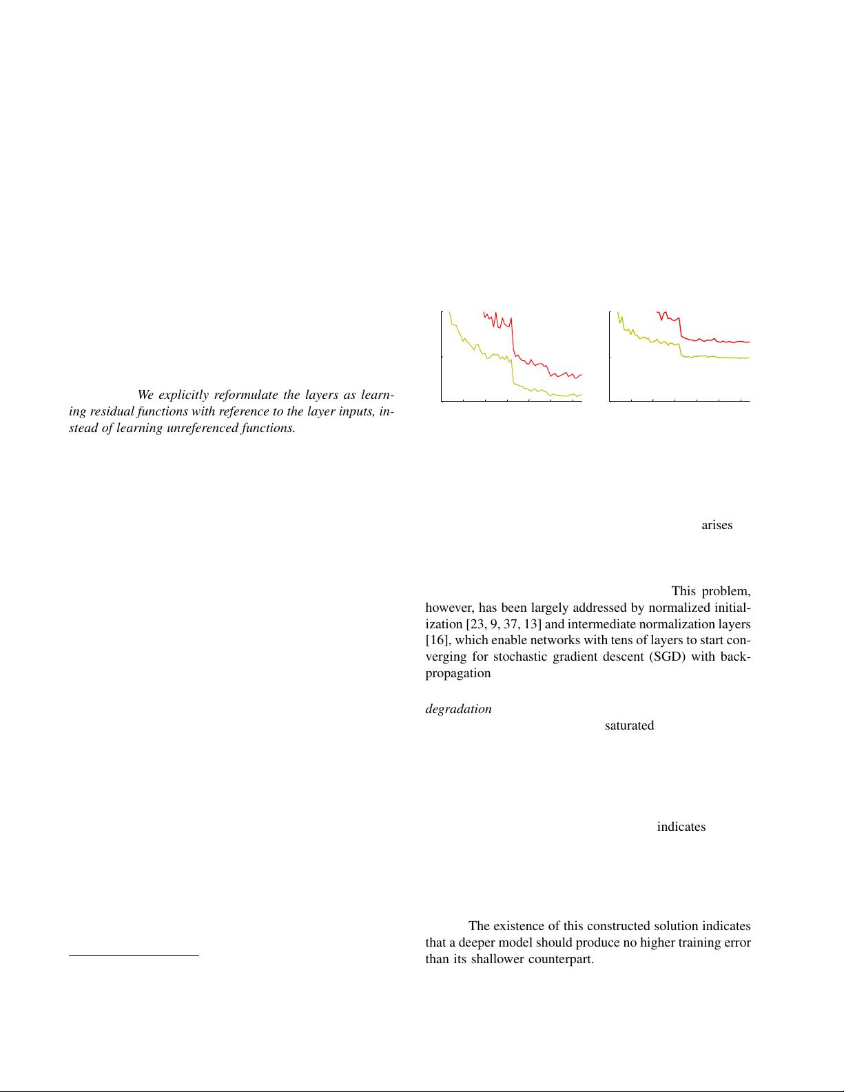
Figure 1. Training error (left) and test error (right) on CIFAR-10

with 20-layer and 56-layer “plain” networks. The deeper network

has higher training error, and thus test error. Similar phenomena

on ImageNet is presented in Fig. 4.

greatly beneﬁted from very deep models.

Driven by the signiﬁcance of depth, a question arises: Is

learning better networks as easy as stacking more layers?

An obstacle to answering this question was the notorious

problem of vanishing/exploding gradients [1, 9], which

hamper convergence from the beginning. This problem,

however, has been largely addressed by normalized initial-

ization [23, 9, 37, 13] and intermediate normalization layers

[16], which enable networks with tens of layers to start con-

verging for stochastic gradient descent (SGD) with back-

propagation [22].

When deeper networks are able to start converging, a

degradation problem has been exposed: with the network

depth increasing, accuracy gets saturated (which might be

unsurprising) and then degrades rapidly. Unexpectedly,

such degradation is not caused by overﬁtting, and adding

more layers to a suitably deep model leads to higher train-

ing error, as reported in [11, 42] and thoroughly veriﬁed by

our experiments. Fig. 1 shows a typical example.

The degradation (of training accuracy) indicates that not

all systems are similarly easy to optimize. Let us consider a

shallower architecture and its deeper counterpart that adds

more layers onto it. There exists a solution by construction

to the deeper model: the added layers are identity mapping,

and the other layers are copied from the learned shallower

model. The existence of this constructed solution indicates

that a deeper model should produce no higher training error

than its shallower counterpart. But experiments show that

our current solvers on hand are unable to ﬁnd solutions that

arXiv:1512.03385v1 [cs.CV] 10 Dec 2015

identity

weight layer

relu

F(x)+x

F(x)

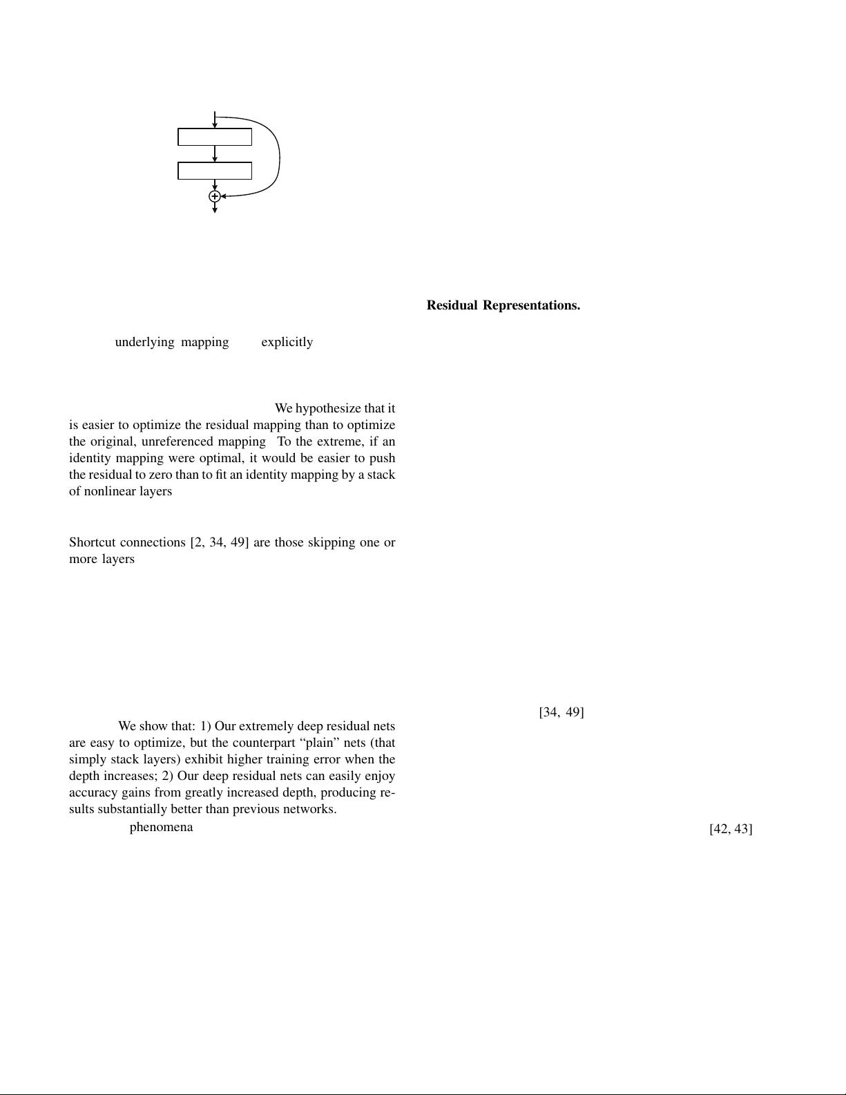
Figure 2. Residual learning: a building block.

are comparably good or better than the constructed solution

(or unable to do so in feasible time).

In this paper, we address the degradation problem by

introducing a deep residual learning framework. In-

stead of hoping each few stacked layers directly ﬁt a

desired underlying mapping, we explicitly let these lay-

ers ﬁt a residual mapping. Formally, denoting the desired

underlying mapping as H(x), we let the stacked nonlinear

layers ﬁt another mapping of F(x):=H(x)  x. The orig-

inal mapping is recast into F(x)+x. We hypothesize that it

is easier to optimize the residual mapping than to optimize

the original, unreferenced mapping. To the extreme, if an

identity mapping were optimal, it would be easier to push

the residual to zero than to ﬁt an identity mapping by a stack

of nonlinear layers.

The formulation of F(x)+x can be realized by feedfor-

ward neural networks with “shortcut connections” (Fig. 2).

Shortcut connections [2, 34, 49] are those skipping one or

more layers. In our case, the shortcut connections simply

perform identity mapping, and their outputs are added to

the outputs of the stacked layers (Fig. 2). Identity short-

cut connections add neither extra parameter nor computa-

tional complexity. The entire network can still be trained

end-to-end by SGD with backpropagation, and can be eas-

ily implemented using common libraries (e.g., Caffe [19])

without modifying the solvers.

We present comprehensive experiments on ImageNet

[36] to show the degradation problem and evaluate our

method. We show that: 1) Our extremely deep residual nets

are easy to optimize, but the counterpart “plain” nets (that

simply stack layers) exhibit higher training error when the

depth increases; 2) Our deep residual nets can easily enjoy

accuracy gains from greatly increased depth, producing re-

sults substantially better than previous networks.

Similar phenomena are also shown on the CIFAR-10 set

[20], suggesting that the optimization difﬁculties and the

effects of our method are not just akin to a particular dataset.

We present successfully trained models on this dataset with

over 100 layers, and explore models with over 1000 layers.

On the ImageNet classiﬁcation dataset [36], we obtain

excellent results by extremely deep residual nets. Our 152-

layer residual net is the deepest network ever presented on

ImageNet, while still having lower complexity than VGG

nets [41]. Our ensemble has 3.57% top-5 error on the

ImageNet test set, and won the 1st place in the ILSVRC

2015 classiﬁcation competition. The extremely deep rep-

resentations also have excellent generalization performance

on other recognition tasks, and lead us to further win the

1st places on: ImageNet detection, ImageNet localization,

COCO detection, and COCO segmentation in ILSVRC &

COCO 2015 competitions. This strong evidence shows that

the residual learning principle is generic, and we expect that

it is applicable in other vision and non-vision problems.

2. Related Work

Residual Representations. In image recognition, VLAD

[18] is a representation that encodes by the residual vectors

with respect to a dictionary, and Fisher Vector [30] can be

formulated as a probabilistic version [18] of VLAD. Both

of them are powerful shallow representations for image re-

trieval and classiﬁcation [4, 48]. For vector quantization,

encoding residual vectors [17] is shown to be more effec-

tive than encoding original vectors.

In low-level vision and computer graphics, for solv-

ing Partial Differential Equations (PDEs), the widely used

Multigrid method [3] reformulates the system as subprob-

lems at multiple scales, where each subproblem is respon-

sible for the residual solution between a coarser and a ﬁner

scale. An alternative to Multigrid is hierarchical basis pre-

conditioning [45, 46], which relies on variables that repre-

sent residual vectors between two scales. It has been shown

[3, 45, 46] that these solvers converge much faster than stan-

dard solvers that are unaware of the residual nature of the

solutions. These methods suggest that a good reformulation

or preconditioning can simplify the optimization.

Shortcut Connections. Practices and theories that lead to

shortcut connections [2, 34, 49] have been studied for a long

time. An early practice of training multi-layer perceptrons

(MLPs) is to add a linear layer connected from the network

input to the output [34, 49]. In [44, 24], a few interme-

diate layers are directly connected to auxiliary classiﬁers

for addressing vanishing/exploding gradients. The papers

of [39, 38, 31, 47] propose methods for centering layer re-

sponses, gradients, and propagated errors, implemented by

shortcut connections. In [44], an “inception” layer is com-

posed of a shortcut branch and a few deeper branches.

Concurrent with our work, “highway networks” [42, 43]

present shortcut connections with gating functions [15].

These gates are data-dependent and have parameters, in

contrast to our identity shortcuts that are parameter-free.

When a gated shortcut is “closed” (approaching zero), the

layers in highway networks represent non-residual func-

tions. On the contrary, our formulation always learns

residual functions; our identity shortcuts are never closed,

and all information is always passed through, with addi-

tional residual functions to be learned. In addition, high-

way networks have not demonstrated accuracy gains with

extremely increased depth (e.g., over 100 layers).

3. Deep Residual Learning

3.1. Residual Learning

Let us consider H(x) as an underlying mapping to be

ﬁt by a few stacked layers (not necessarily the entire net),

with x denoting the inputs to the ﬁrst of these layers. If one

hypothesizes that multiple nonlinear layers can asymptoti-

cally approximate complicated functions

, then it is equiv-

alent to hypothesize that they can asymptotically approxi-

mate the residual functions, i.e., H(x)  x (assuming that

the input and output are of the same dimensions). So

rather than expect stacked layers to approximate H(x), we

explicitly let these layers approximate a residual function

F(x):=H(x)  x. The original function thus becomes

F(x)+x. Although both forms should be able to asymptot-

ically approximate the desired functions (as hypothesized),

the ease of learning might be different.

This reformulation is motivated by the counterintuitive

phenomena about the degradation problem (Fig. 1, left). As

we discussed in the introduction, if the added layers can

be constructed as identity mappings, a deeper model should

have training error no greater than its shallower counter-

part. The degradation problem suggests that the solvers

might have difﬁculties in approximating identity mappings

by multiple nonlinear layers. With the residual learning re-

formulation, if identity mappings are optimal, the solvers

may simply drive the weights of the multiple nonlinear lay-

ers toward zero to approach identity mappings.

In real cases, it is unlikely that identity mappings are op-

timal, but our reformulation may help to precondition the

problem. If the optimal function is closer to an identity

mapping than to a zero mapping, it should be easier for the

solver to ﬁnd the perturbations with reference to an identity

mapping, than to learn the function as a new one. We show

by experiments (Fig. 7) that the learned residual functions in

general have small responses, suggesting that identity map-

pings provide reasonable preconditioning.

3.2. Identity Mapping by Shortcuts

We adopt residual learning to every few stacked layers.

A building block is shown in Fig. 2. Formally, in this paper

we consider a building block deﬁned as:

y = F(x, {W

})+x. (1)

Here x and y are the input and output vectors of the lay-

ers considered. The function F(x , {W

}) represents the

residual mapping to be learned. For the example in Fig. 2

that has two layers, F = W

(W

x) in which  denotes

This hypothesis, however, is still an open question. See [28].

ReLU [29] and the biases are omitted for simplifying no-

tations. The operation F + x is performed by a shortcut

connection and element-wise addition. We adopt the sec-

ond nonlinearity after the addition (i.e., (y), see Fig. 2).

The shortcut connections in Eqn.(1) introduce neither ex-

tra parameter nor computation complexity. This is not only

attractive in practice but also important in our comparisons

between plain and residual networks. We can fairly com-

pare plain/residual networks that simultaneously have the

same number of parameters, depth, width, and computa-

tional cost (except for the negligible element-wise addition).

The dimensions of x and F must be equal in Eqn.(1).

If this is not the case (e.g., when changing the input/output

channels), we can perform a linear projection W

by the

shortcut connections to match the dimensions:

y = F(x, {W

})+W

x. (2)

We can also use a square matrix W

in Eqn.(1). But we will

show by experiments that the identity mapping is sufﬁcient

for addressing the degradation problem and is economical,

and thus W

is only used when matching dimensions.

The form of the residual function F is ﬂexible. Exper-

iments in this paper involve a function F that has two or

three layers (Fig. 5), while more layers are possible. But if

F has only a single layer, Eqn.(1) is similar to a linear layer:

y = W

x + x, for which we have not observed advantages.

We also note that although the above notations are about

fully-connected layers for simplicity, they are applicable to

convolutional layers. The function F(x, {W

}) can repre-

sent multiple convolutional layers. The element-wise addi-

tion is performed on two feature maps, channel by channel.

3.3. Network Architectures

We have tested various plain/residual nets, and have ob-

served consistent phenomena. To provide instances for dis-

cussion, we describe two models for ImageNet as follows.

Plain Network. Our plain baselines (Fig. 3, middle) are

mainly inspired by the philosophy of VGG nets [41] (Fig. 3,

left). The convolutional layers mostly have 3⇥3 ﬁlters and

follow two simple design rules: (i) for the same output

feature map size, the layers have the same number of ﬁl-

ters; and (ii) if the feature map size is halved, the num-

ber of ﬁlters is doubled so as to preserve the time com-

plexity per layer. We perform downsampling directly by

convolutional layers that have a stride of 2. The network

ends with a global average pooling layer and a 1000-way

fully-connected layer with softmax. The total number of

weighted layers is 34 in Fig. 3 (middle).

It is worth noticing that our model has fewer ﬁlters and

lower complexity than VGG nets [41] (Fig. 3, left). Our 34-

layer baseline has 3.6 billion FLOPs (multiply-adds), which

is only 18% of VGG-19 (19.6 billion FLOPs).

剩余11页未读，继续阅读

评论收藏

内容反馈

不脱发的程序猿

粉丝: 26w+
资源: 5887

Deep Residual Learning for Image Recognition.pdf

最新资源

Deep Residual Learning for Image Recognition.pdf

【7】Deep residual learning for image recognition.pdf

Deep Residual Learning for Image Recognition

inet--ResNet--Deep Residual Learning for Image Recognition.pdf

Deep Residual Learning for Image Recognition原版及翻译及笔记

Deep Residual Learning for Image Recognition 机翻

paper reading:Deep Residual Learning for Image Recognition

Deep Residual Learning for Image Recognition 深度残差网络论文笔记

Deep Residual Learning for Image Recognition（七月在线DL翻译组2017.4）

Deep Residual Learning for Image Recognition浅读与实现

resnet ppt refer to Deep Residual Learning for Image Recognition

论文精读-Deep Residual Learning for Image Recognition

人工智能相关论文综合.zip

resnet学习.zip

十种流行网络在cifar-10数据集上的应用

基于深度学习的人脸识别技术在学习效果评价中的应用研究.pdf

深度残差收缩网络和极端随机森林.zip

基于深度学习的入侵检测方法.pdf

Deep Learning with Theano [2017]

Introduction to Deep Learning Business Applications for Developers: From

文献打包-An Introduction Of Densely Connected Convolutional Networks

基于深度学习的交通标志识别方法研究.pdf

Python实现多人脸识别系统.zip

CNN卷积神经网络资料汇总1

吴恩达深度学习课程第四课相关论文

Deep learing 论文合集，一条小白到发论文的必须道路！

Academic+Phrasebank+2021+Edition+_中英文对照.pdf

YOLO v1 ~ YOLO v5 论文解读和实现细节

最新资源