没有合适的资源?快使用搜索试试~ 我知道了~
资源推荐
资源详情
资源评论

Gradient descent is one of the most popular algorithms to perform optimization and by far
the most common way to optimize neural networks. At the same time, every state-of-the-
art Deep Learning library contains implementations of various algorithms to optimize
gradient descent (e.g. , , and documentation). These algorithms,
however, are often used as black-box optimizers, as practical explanations of their
strengths and weaknesses are hard to come by.
This blog post aims at providing you with intuitions towards the behaviour of different
algorithms for optimizing gradient descent that will help you put them to use. We are first
going to look at the different variants of gradient descent. We will then briefly summarize
challenges during training. Subsequently, we will introduce the most common optimization
Adadelta
RMSprop
Adam
Visualization of algorithms
Which optimizer to choose?
Parallelizing and distributing SGD
Hogwild!
Downpour SGD
Delay-tolerant Algorithms for SGD
TensorFlow
Elasic Averaging SGD
Additional strategies for optimizing SGD
Shuffling and Curriculum Learning
Batch normalization
Early Stopping
Gradient noise
Conclusion
References
lasagne's caffe's keras'

algorithms by showing their motivation to resolve these challenges and how this leads to
the derivation of their update rules. We will also take a short look at algorithms and
architectures to optimize gradient descent in a parallel and distributed setting. Finally, we
will consider additional strategies that are helpful for optimizing gradient descent.
Gradient descent is a way to minimize an objective function parameterized by a
model's parameters by updating the parameters in the opposite direction of the
gradient of the objective function w.r.t. to the parameters. The learning rate
determines the size of the steps we take to reach a (local) minimum. In other words, we
follow the direction of the slope of the surface created by the objective function downhill
until we reach a valley. If you are unfamiliar with gradient descent, you can find a good
introduction on optimizing neural networks .
Gradient descent variants
There are three variants of gradient descent, which differ in how much data we use to
compute the gradient of the objective function. Depending on the amount of data, we
make a trade-off between the accuracy of the parameter update and the time it takes to
perform an update.
Batch gradient descent
Vanilla gradient descent, aka batch gradient descent, computes the gradient of the cost
function w.r.t. to the parameters for the entire training dataset:
.
As we need to calculate the gradients for the whole dataset to perform just
one
update,
batch gradient descent can be very slow and is intractable for datasets that don't fit in
memory. Batch gradient descent also doesn't allow us to update our model
online
, i.e. with
new examples on-the-fly.
In code, batch gradient descent looks something like this:
J
(
θ
)
θ
∈
ℝ
d
J
(
θ
)
∇
θ
η
here
θ
θ
=
θ
−
η
⋅
J
(
θ
)
∇
θ

for i in range(nb_epochs):
params_grad = evaluate_gradient(loss_function, data, params)
params = params - learning_rate * params_grad
For a pre-defined number of epochs, we first compute the gradient vector weights_grad
of the loss function for the whole dataset w.r.t. our parameter vector params. Note that
state-of-the-art deep learning libraries provide automatic differentiation that efficiently
computes the gradient w.r.t. some parameters. If you derive the gradients yourself, then
gradient checking is a good idea. (See for some great tips on how to check gradients
properly.)
We then update our parameters in the direction of the gradients with the learning rate
determining how big of an update we perform. Batch gradient descent is guaranteed to
converge to the global minimum for convex error surfaces and to a local minimum for non-
convex surfaces.
Stochastic gradient descent
Stochastic gradient descent (SGD) in contrast performs a parameter update for
each
training example and label :
.
Batch gradient descent performs redundant computations for large datasets, as it
recomputes gradients for similar examples before each parameter update. SGD does away
with this redundancy by performing one update at a time. It is therefore usually much
faster and can also be used to learn online.
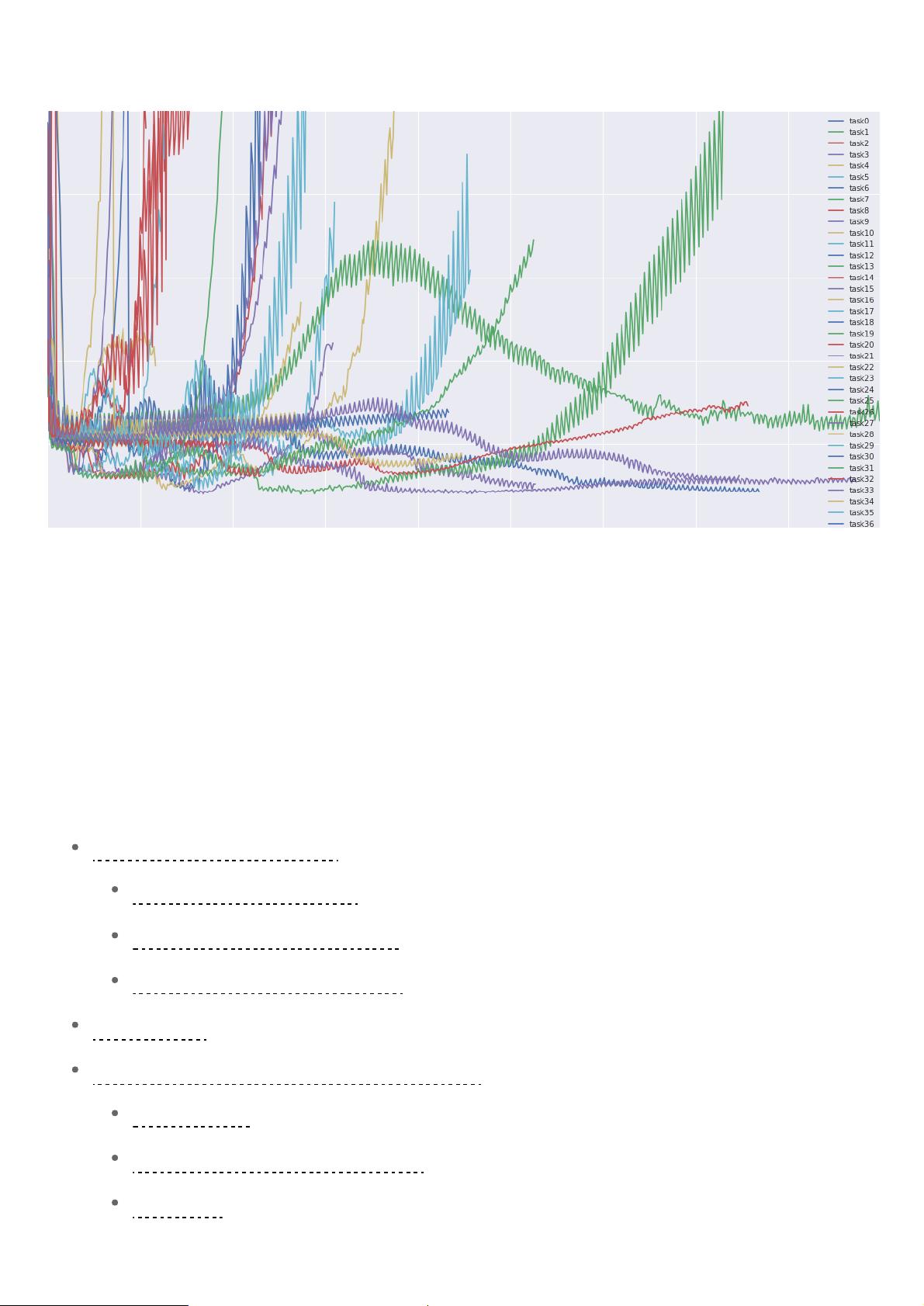
SGD performs frequent updates with a high variance that cause the objective function to
fluctuate heavily as in Image 1.
here
x
(
i
)
y
(
i
)
θ
=
θ
−
η
⋅
J
(
θ
; ; )
∇
θ
x
(
i
)
y
(
i
)
剩余20页未读,继续阅读
资源评论

- #完美解决问题
- #运行顺畅
- #内容详尽
- #全网独家
- #注释完整
Leo青山
- 粉丝: 1
- 资源: 1
上传资源 快速赚钱
 我的内容管理
展开
 我的资源
快来上传第一个资源
 我的收益 登录查看自己的收益
 我的积分
登录查看自己的积分
 我的C币
登录后查看C币余额
 我的收藏
我的收藏  我的下载
我的下载  下载帮助
下载帮助

 前往需求广场,查看用户热搜
最新资源
- 【SEC-2025行业研究报告】Form 10-K Blue Owl Credit Income Corp. .pdf
- 【SEC-2025行业研究报告】Form 10-K CEDAR REALTY TRUST, INC. .pdf
- 【SEC-2025行业研究报告】Form 10-K ChromaDex Corp. .pdf
- 【SEC-2025行业研究报告】Form 10-K BRIGHTHOUSE LIFE INSURANCE Co .pdf
- 【SEC-2025行业研究报告】Form 10-K CPI Card Group Inc. .pdf
- 【SEC-2025行业研究报告】Form 10-K Custom Truck One Source, Inc. .pdf
- 【SEC-2025行业研究报告】Form 10-K Crexendo, Inc. .pdf
- 【SEC-2025行业研究报告】Form 10-K Cyclerion Therapeutics, Inc. .pdf
- 【SEC-2025行业研究报告】Form 10-K Dave Inc. DE .pdf
- 【SEC-2025行业研究报告】Form 10-K Emergent BioSolutions Inc. .pdf
- 【SEC-2025行业研究报告】Form 10-K Eos Energy Enterprises, Inc. .pdf
- 【SEC-2025行业研究报告】Form 10-K Evolus, Inc. .pdf
- 【SEC-2025行业研究报告】Form 10-K FLAGSTAR FINANCIAL, INC. .pdf
- 【SEC-2025行业研究报告】Form 10-Q NKGen Biotech, Inc. .pdf
- 【SEC-2025行业研究报告】Form 10-Q DONALDSON Co INC .pdf
- 【SEC-2025行业研究报告】Form 10-K Flutter Entertainment plc .pdf
资源上传下载、课程学习等过程中有任何疑问或建议,欢迎提出宝贵意见哦~我们会及时处理!
点击此处反馈


安全验证
文档复制为VIP权益,开通VIP直接复制
 信息提交成功


