没有合适的资源?快使用搜索试试~ 我知道了~
A Tutorial on Principal Component Analysis [2014]
需积分: 23 8 下载量 20 浏览量
2018-11-26
21:38:56
上传
评论
收藏 377KB PDF 举报
温馨提示
试读
12页
A Tutorial on Principal Component Analysis by Jonathon Shlens. 2014年版。英文。
资源推荐
资源详情
资源评论
A Tutorial on Principal Component Analysis
Jonathon Shlens
∗
Google Research
Mountain View, CA 94043
(Dated: April 7, 2014; Version 3.02)
Principal component analysis (PCA) is a mainstay of modern data analysis - a black box that is widely used
but (sometimes) poorly understood. The goal of this paper is to dispel the magic behind this black box. This
manuscript focuses on building a solid intuition for how and why principal component analysis works. This
manuscript crystallizes this knowledge by deriving from simple intuitions, the mathematics behind PCA. This
tutorial does not shy away from explaining the ideas informally, nor does it shy away from the mathematics. The
hope is that by addressing both aspects, readers of all levels will be able to gain a better understanding of PCA as
well as the when, the how and the why of applying this technique.
I. INTRODUCTION
Principal component analysis (PCA) is a standard tool in mod-
ern data analysis - in diverse fields from neuroscience to com-
puter graphics - because it is a simple, non-parametric method
for extracting relevant information from confusing data sets.
With minimal effort PCA provides a roadmap for how to re-
duce a complex data set to a lower dimension to reveal the
sometimes hidden, simplified structures that often underlie it.
The goal of this tutorial is to provide both an intuitive feel for
PCA, and a thorough discussion of this topic. We will begin
with a simple example and provide an intuitive explanation
of the goal of PCA. We will continue by adding mathemati-
cal rigor to place it within the framework of linear algebra to
provide an explicit solution. We will see how and why PCA
is intimately related to the mathematical technique of singular
value decomposition (SVD). This understanding will lead us
to a prescription for how to apply PCA in the real world and an
appreciation for the underlying assumptions. My hope is that
a thorough understanding of PCA provides a foundation for
approaching the fields of machine learning and dimensional
reduction.
The discussion and explanations in this paper are informal in
the spirit of a tutorial. The goal of this paper is to educate.
Occasionally, rigorous mathematical proofs are necessary al-
though relegated to the Appendix. Although not as vital to the
tutorial, the proofs are presented for the adventurous reader
who desires a more complete understanding of the math. My
only assumption is that the reader has a working knowledge
of linear algebra. My goal is to provide a thorough discussion
by largely building on ideas from linear algebra and avoiding
challenging topics in statistics and optimization theory (but
see Discussion). Please feel free to contact me with any sug-
gestions, corrections or comments.
∗
Electronic address: jonathon.shlens@gmail.com
II. MOTIVATION: A TOY EXAMPLE
Here is the perspective: we are an experimenter. We are trying
to understand some phenomenon by measuring various quan-
tities (e.g. spectra, voltages, velocities, etc.) in our system.
Unfortunately, we can not figure out what is happening be-
cause the data appears clouded, unclear and even redundant.
This is not a trivial problem, but rather a fundamental obstacle
in empirical science. Examples abound from complex sys-
tems such as neuroscience, web indexing, meteorology and
oceanography - the number of variables to measure can be
unwieldy and at times even deceptive, because the underlying
relationships can often be quite simple.
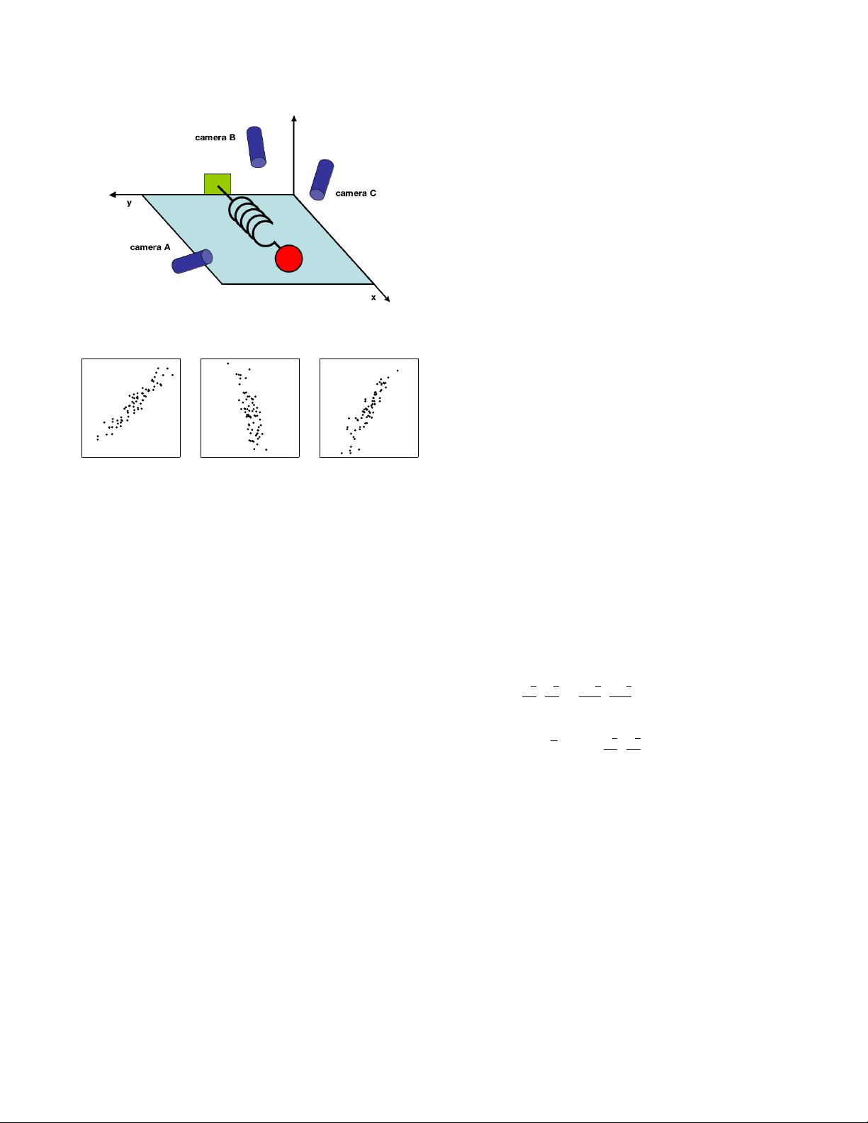
Take for example a simple toy problem from physics dia-
grammed in Figure 1. Pretend we are studying the motion
of the physicist’s ideal spring. This system consists of a ball
of mass m attached to a massless, frictionless spring. The ball
is released a small distance away from equilibrium (i.e. the
spring is stretched). Because the spring is ideal, it oscillates
indefinitely along the x-axis about its equilibrium at a set fre-
quency.
This is a standard problem in physics in which the motion
along the x direction is solved by an explicit function of time.
In other words, the underlying dynamics can be expressed as
a function of a single variable x.
However, being ignorant experimenters we do not know any
of this. We do not know which, let alone how many, axes
and dimensions are important to measure. Thus, we decide to
measure the ball’s position in a three-dimensional space (since
we live in a three dimensional world). Specifically, we place
three movie cameras around our system of interest. At 120 Hz
each movie camera records an image indicating a two dimen-
sional position of the ball (a projection). Unfortunately, be-
cause of our ignorance, we do not even know what are the real
x, y and z axes, so we choose three camera positions
~
a,
~
b and
~
c
at some arbitrary angles with respect to the system. The angles
between our measurements might not even be 90
o
! Now, we
record with the cameras for several minutes. The big question
remains: how do we get from this data set to a simple equation
arXiv:1404.1100v1 [cs.LG] 3 Apr 2014
2
camera A camera B camera C
FIG. 1 A toy example. The position of a ball attached to an oscillat-
ing spring is recorded using three cameras A, B and C. The position
of the ball tracked by each camera is depicted in each panel below.
of x?
We know a-priori that if we were smart experimenters, we
would have just measured the position along the x-axis with
one camera. But this is not what happens in the real world.
We often do not know which measurements best reflect the
dynamics of our system in question. Furthermore, we some-
times record more dimensions than we actually need.
Also, we have to deal with that pesky, real-world problem of
noise. In the toy example this means that we need to deal
with air, imperfect cameras or even friction in a less-than-ideal
spring. Noise contaminates our data set only serving to obfus-
cate the dynamics further. This toy example is the challenge
experimenters face everyday. Keep this example in mind as
we delve further into abstract concepts. Hopefully, by the end
of this paper we will have a good understanding of how to
systematically extract x using principal component analysis.
III. FRAMEWORK: CHANGE OF BASIS
The goal of principal component analysis is to identify the
most meaningful basis to re-express a data set. The hope is
that this new basis will filter out the noise and reveal hidden
structure. In the example of the spring, the explicit goal of
PCA is to determine: “the dynamics are along the x-axis.” In
other words, the goal of PCA is to determine that
ˆ
x, i.e. the
unit basis vector along the x-axis, is the important dimension.
Determining this fact allows an experimenter to discern which
dynamics are important, redundant or noise.
A. A Naive Basis
With a more precise definition of our goal, we need a more
precise definition of our data as well. We treat every time
sample (or experimental trial) as an individual sample in our
data set. At each time sample we record a set of data consist-
ing of multiple measurements (e.g. voltage, position, etc.). In
our data set, at one point in time, camera A records a corre-
sponding ball position (x
A
,y
A
). One sample or trial can then
be expressed as a 6 dimensional column vector
~
X =
x
A
y
A
x
B
y
B
x
C
y
C
where each camera contributes a 2-dimensional projection of
the ball’s position to the entire vector
~
X. If we record the ball’s
position for 10 minutes at 120 Hz, then we have recorded 10×
60 ×120 = 72000 of these vectors.
With this concrete example, let us recast this problem in ab-
stract terms. Each sample
~
X is an m-dimensional vector,
where m is the number of measurement types. Equivalently,
every sample is a vector that lies in an m-dimensional vec-
tor space spanned by some orthonormal basis. From linear
algebra we know that all measurement vectors form a linear
combination of this set of unit length basis vectors. What is
this orthonormal basis?
This question is usually a tacit assumption often overlooked.
Pretend we gathered our toy example data above, but only
looked at camera A. What is an orthonormal basis for (x
A
,y
A
)?
A naive choice would be {(1,0),(0,1)}, but why select this
basis over {(
√
2
2
,
√
2
2
),(
−
√
2
2
,
−
√
2
2
)}or any other arbitrary rota-
tion? The reason is that the naive basis reflects the method we
gathered the data. Pretend we record the position (2, 2). We
did not record 2
√
2 in the (
√
2
2
,
√
2
2
) direction and 0 in the per-
pendicular direction. Rather, we recorded the position (2, 2)
on our camera meaning 2 units up and 2 units to the left in our
camera window. Thus our original basis reflects the method
we measured our data.
How do we express this naive basis in linear algebra? In the
two dimensional case, {(1,0),(0,1)} can be recast as individ-
ual row vectors. A matrix constructed out of these row vectors
is the 2 ×2 identity matrix I. We can generalize this to the m-
dimensional case by constructing an m ×m identity matrix
B =
b
1
b
2
.
.
.
b
m
=
1 0 ··· 0
0 1 ··· 0
.
.
.
.
.
.
.
.
.
.
.
.
0 0 ··· 1
= I
where each row is an orthornormal basis vector b
i
with m
components. We can consider our naive basis as the effective
starting point. All of our data has been recorded in this basis
3
and thus it can be trivially expressed as a linear combination
of {b
i
}.
B. Change of Basis
With this rigor we may now state more precisely what PCA
asks: Is there another basis, which is a linear combination of
the original basis, that best re-expresses our data set?
A close reader might have noticed the conspicuous addition of
the word linear. Indeed, PCA makes one stringent but power-
ful assumption: linearity. Linearity vastly simplifies the prob-
lem by restricting the set of potential bases. With this assump-
tion PCA is now limited to re-expressing the data as a linear
combination of its basis vectors.
Let X be the original data set, where each column is a single
sample (or moment in time) of our data set (i.e.
~
X). In the toy
example X is an m ×n matrix where m = 6 and n = 72000.
Let Y be another m ×n matrix related by a linear transfor-
mation P. X is the original recorded data set and Y is a new
representation of that data set.
PX = Y (1)
Also let us define the following quantities.
1
• p
i
are the rows of P
• x
i
are the columns of X (or individual
~
X).
• y
i
are the columns of Y.
Equation 1 represents a change of basis and thus can have
many interpretations.
1. P is a matrix that transforms X into Y.
2. Geometrically, P is a rotation and a stretch which again
transforms X into Y.
3. The rows of P,
{
p
1
,...,p
m
}
, are a set of new basis vec-
tors for expressing the columns of X.
The latter interpretation is not obvious but can be seen by writ-
ing out the explicit dot products of PX.
PX =
p
1
.
.
.
p
m
x
1
··· x
n
Y =
p
1
·x
1
··· p
1
·x
n
.
.
.
.
.
.
.
.
.
p
m
·x
1
··· p
m
·x
n
1
In this section x
i
and y
i
are column vectors, but be forewarned. In all other
sections x
i
and y
i
are row vectors.
We can note the form of each column of Y.
y
i
=
p
1
·x
i
.
.
.
p
m
·x
i
We recognize that each coefficient of y
i
is a dot-product of
x
i
with the corresponding row in P. In other words, the j
th
coefficient of y
i
is a projection on to the j
th
row of P. This is
in fact the very form of an equation where y
i
is a projection
on to the basis of
{
p
1
,...,p
m
}
. Therefore, the rows of P are a
new set of basis vectors for representing of columns of X.
C. Questions Remaining
By assuming linearity the problem reduces to finding the ap-
propriate change of basis. The row vectors
{
p
1
,...,p
m
}
in
this transformation will become the principal components of
X. Several questions now arise.
• What is the best way to re-express X?
• What is a good choice of basis P?
These questions must be answered by next asking ourselves
what features we would like Y to exhibit. Evidently, addi-
tional assumptions beyond linearity are required to arrive at
a reasonable result. The selection of these assumptions is the
subject of the next section.
IV. VARIANCE AND THE GOAL
Now comes the most important question: what does best ex-
press the data mean? This section will build up an intuitive
answer to this question and along the way tack on additional
assumptions.
A. Noise and Rotation
Measurement noise in any data set must be low or else, no
matter the analysis technique, no information about a signal
can be extracted. There exists no absolute scale for noise but
rather all noise is quantified relative to the signal strength. A
common measure is the signal-to-noise ratio (SNR), or a ratio
of variances σ
2
,
SNR =
σ
2
signal
σ
2
noise
.
A high SNR ( 1) indicates a high precision measurement,
while a low SNR indicates very noisy data.
剩余11页未读,继续阅读
资源评论
larry_dongy
- 粉丝: 563
- 资源: 18
上传资源 快速赚钱
- 我的内容管理 展开
- 我的资源 快来上传第一个资源
- 我的收益 登录查看自己的收益
- 我的积分 登录查看自己的积分
- 我的C币 登录后查看C币余额
- 我的收藏
- 我的下载
- 下载帮助
安全验证
文档复制为VIP权益,开通VIP直接复制
信息提交成功