没有合适的资源?快使用搜索试试~ 我知道了~
polynomial_operations.pdf
1.该资源内容由用户上传,如若侵权请联系客服进行举报
2.虚拟产品一经售出概不退款(资源遇到问题,请及时私信上传者)
版权申诉
0 下载量 92 浏览量
2023-06-18
13:15:20
上传
评论
收藏 339KB PDF 举报
温馨提示
试读
11页
polynomial_operations.pdf
资源推荐
资源详情
资源评论
Polynomials:
Representation, Evaluation, Operations
MATH2070: Numerical Methods in Scientific Computing I
Location: http://people.sc.fsu.edu/∼jburkardt/classes/math2070 2019/polynomial operations/polynomial operations.pdf
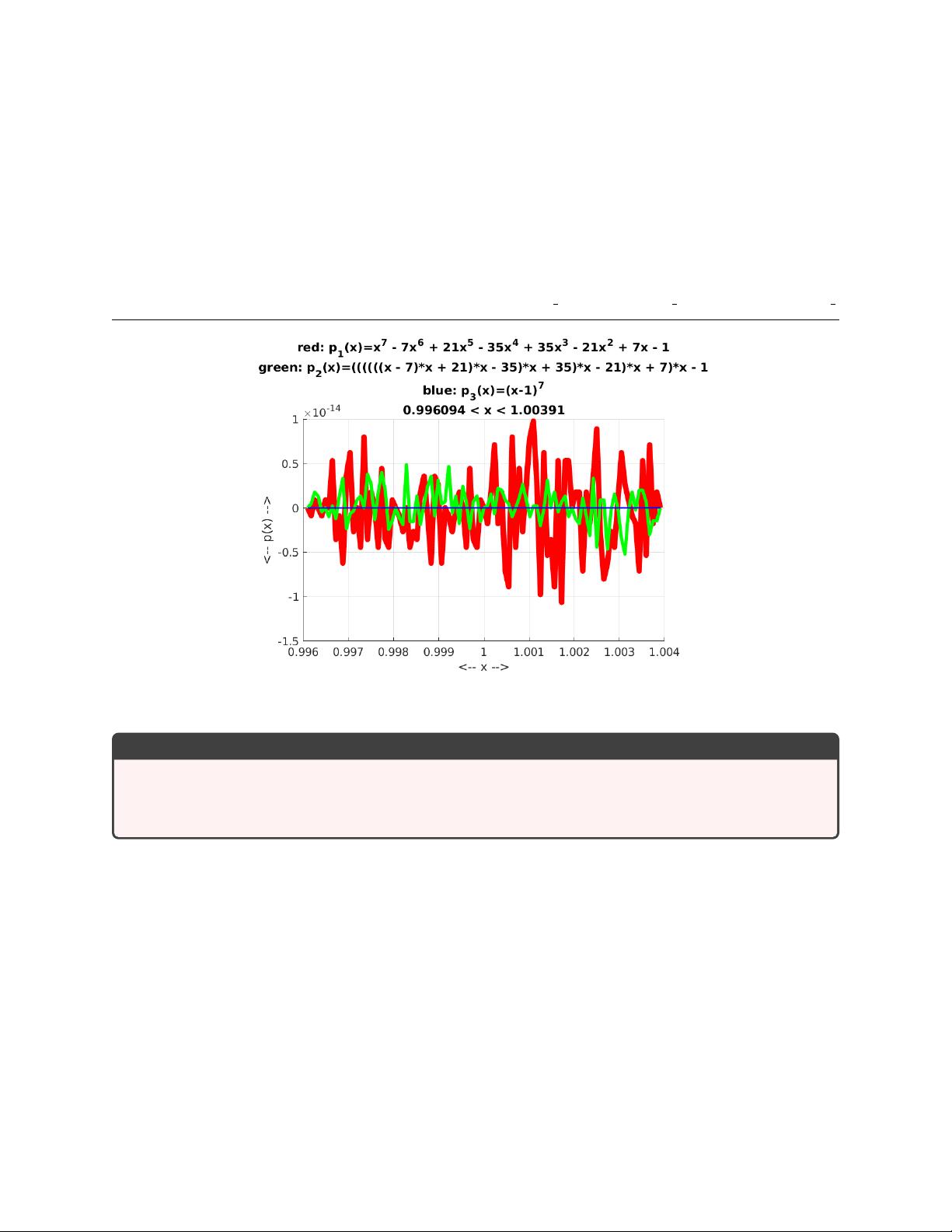
Evaluating three representations of the same polynomial.
Polynomial Computations
• What choices are there for representing a polynomial?
• What is an efficient evaluation procedure?
• How do we add, multiply, divide, differentiate, and integrate?
A (real) polynomial of degree d can be defined in power form as
p(x) = c
0
+ c
1
x + c
2
x
2
+ ... + c
d
x
d
Mathematical power form (0-based)
where the quantities c
i
are real numbers known as the coefficients of the polynomial. Here, the subscript of
the coefficient c
i
matches the corresponding power x
i
. This is the most natural way to describe a polynomial.
We assume that c
d
is not 0, otherwise the polynomial actually has a degree lower than d.
1 Power form (1-based)
MATLAB does not allow the use of 0 as an array index. The simplest way to deal with this issue is to use
a “1-based” power form, in which c
i+1
multiplies x
i
:
p(x) = c
1
+ c
2
x + c
3
x
2
+ ... + c
d+1
x
d
power form (1-based)
1
Because it is still pretty easy to think about polynomials this way, this is the form that we will prefer for
most of the following discussion.
Thus, the degree-3 polynomial
p(x) = 1.1 + 3.3x
2
− 4.44x
3
could be stored as a MATLAB array of 4 entries:
1 c = [ 1 . 1 , 0 . 0 , 3 . 3 , 4.44 ]
2 Print a polynomial
If we want to print out a polynomial, we could just print the vector of coefficients c. It is much more
intelligible to try to reproduce the full mathematical form, if possible. Here is a very basic example that
suggest how we might do this:
1 function p o l y p r i n t ( c )
2 d = length ( c ) − 1 ;
3 f or i = 0 : d
4 f p r i n tf ( ’%g xˆ%d\n ’ , c ( i +1) , i ) ;
5 end
6 return
7 end
Listing 1: Basic poly print.m code.
While we could work harder to make nicer output, here’s what happens if we call the function to print out
3x
5
− 2x
3
+ x
2
− 5x − 17:
1 c = [ −17 , −5, 1 , −2, 0 , 3 ] ;
2 p o l y p r i n t ( c ) ;
3
4 −17 xˆ0
5 −5 xˆ1
6 1 xˆ2
7 −2 xˆ3
8 0 xˆ4
9 3 xˆ5
Listing 2: Using poly print().
For somewhat nicer output, we could try the fancier function r8poly print(c).
1 c = [ −17 , −5, 1 , −2, 0 , 3 ] ;
2 r 8 p o l y p r i n t ( c ) ;
3
4 p ( x ) = 3.0 0 0000 ∗ xˆ5
5 − 2.0 0 0000 ∗ xˆ4
6 + 1.0 0 0 000 ∗ xˆ2
7 − 5.0 0 0000 ∗ x
8 − 17. 0 000 0 0
Listing 3: Using the fancier r8poly print().
which prints the polynomial in the more traditional form in which the highest power is shown first. It also
omits powers of x with zero coefficient.
2
3 Add two polynomials
Adding two polynomials just means combining coefficients of the same power. The polynomials may have
different degrees; the degree of the sum should be the higher of the two degrees. We can simplify the process
by copying the coefficients of the higher degree polynomial, and then adding the coefficients of the lower
degree polynomial:
1 function c3 = p oly add ( c1 , c2 )
2 d1 = length ( c1 ) − 1 ;
3 d2 = length ( c2 ) − 1 ;
4 d3 = max ( d1 , d2 ) ;
5 c3 = zeros ( d3+1 , 1 ) ;
6
7 i f ( d2 < d1 )
8 c3 = c1 ;
9 f or i = 0 : d2
10 c3 ( i +1) = c3 ( i +1) + c2 ( i +1) ;
11 end
12 e ls e
13 c = c2 ;
14 f or i = 0 : d1
15 c3 ( i +1) = c3 ( i +1) + c1 ( i +1) ;
16 end
17 end
18
19 return
20 end
Listing 4: Polynomial addition.
Why couldn’t we simply say the following?
1 f or i = 0 : d3
2 c3 ( i +1) = c1 ( i +1) + c2 ( i +1) ;
3 end
Listing 5: Explain why this is a bad idea.
4 Multiply two polynomials
Mathematically, if p
3
= p
1
∗ p
2
, then the coefficients of p
3
can be computed by
c
3
k
=
X
i+j=k
c
1
i
c
2
j
0 ≤ k ≤ d
1
+ d
2
So computationally, multiplying two polynomials means computing every possible product c1(i) ∗ c2(j) and
adding that to c3(i + j). But we have to remember to increment our coefficient indices by 1. The degree of
the product will be the sum of the degrees of the factors:
1 function c3 = p o l y m u l t i p l y ( c1 , c2 )
2 d1 = length ( c1 ) − 1 ;
3 d2 = length ( c2 ) − 1 ;
4 d3 = d1 + d2 ;
5 c3 = zeros ( d3+1 , 1 ) ;
6
7 f or i = 0 : d1
8 f or j = 0 : d2
9 c3 ( i+j +1) = c3 ( i+j +1) + c1 ( i +1) ∗ c2 ( j +1) ;
10 end
11 end
3
剩余10页未读,继续阅读
资源评论
卷积神经网络
- 粉丝: 339
- 资源: 8460
上传资源 快速赚钱
- 我的内容管理 展开
- 我的资源 快来上传第一个资源
- 我的收益 登录查看自己的收益
- 我的积分 登录查看自己的积分
- 我的C币 登录后查看C币余额
- 我的收藏
- 我的下载
- 下载帮助
最新资源
- ModStartCMS v8.4.0 框架稳定性持续迭代,修复部分已知问题
- bleder 教室学校学生教育室办公室考试
- 人脸检测-使用OpenCV实现的动漫+漫画人脸检测算法-附项目源码-优质项目实战.zip
- 道路贴图,材质材料免费
- 人脸检测-基于OpenCV+Node.js+WebSockets实现的实时人脸检测应用-附项目源码-优质项目实战.zip
- 一些常见的MySQL死锁案例-mysql-deadlocks-master(源代码+案例+图解说明)
- UE4动画烘焙器-ue4.27
- 新建文件夹.zip
- 1103a2a791bbd96ea98021062e327495b1c422e32fb27e0c2d6404b1bd74b692.gif
- 同城相亲交友php小程序
资源上传下载、课程学习等过程中有任何疑问或建议,欢迎提出宝贵意见哦~我们会及时处理!
点击此处反馈
安全验证
文档复制为VIP权益,开通VIP直接复制
信息提交成功