


2 Programming Question
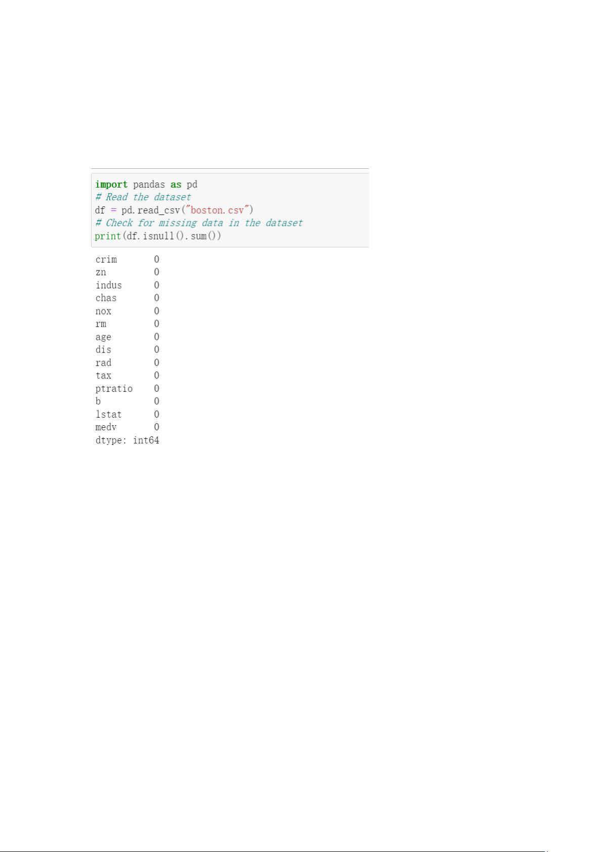
Step 1: use pandas library to check the data in the dataset. Process incomplete
data point such as ’NaN’ or Null’. Briefly summarize the characteristics of
this dataset and guess which is the most relevant attribute for MEDV.

From the df.info() output, we can see that the data types of the columns are as follows:
crim, zn, indus, nox, age, dis, ptratio, b, lstat, and medv are of type float64
chas and rad are of type int64
tax is of type int64
All the columns have 506 non-null values, which means that there are no missing values in the
dataset. This is a good sign as missing values can affect the accuracy of any model built using this
dataset.

From the sorted correlation matrix, we can see that the most relevant attribute for MEDV is
LSTAT with a correlation of -0.737663. This means that as the value of LSTAT increases, the
value of MEDV decreases. The second most relevant attribute is RM with a correlation of
0.695360, which means that as the value of RM increases, the value of MEDV increases.
These two attributes, LSTAT and RM, are likely to be the most important for predicting the
median value of owner-occupied homes in the area of Boston. Other attributes such as ZN, B, and
DIS also have some correlation with MEDV, but the correlation is not as strong as that of LSTAT
and RM.
Step 2: use seaborn library to visualize the dataset. Plot the MEDV distributions
over each attribute. Briefly analyze the characteristics of the attributes and
revise the assumption in Step 1 if necessary.

create a joint plot of LSTAT and MEDV using the seaborn library. The plot will show the
distribution of MEDV with LSTAT and also display a regression line to visualize the relationship
between the two variables. This plot can provide additional insight into the relationship between
LSTAT and MEDV and help us determine if LSTAT is indeed the most relevant attribute for
predicting MEDV.
The distribution of MEDV with LSTAT shows a strong negative linear relationship, meaning that
as the value of LSTAT increases, the value of MEDV decreases. This confirms that LSTAT is
indeed a strong predictor of MEDV.
From the joint plot, we can see that the data points form a clear downward trend and that the
regression line accurately represents this trend. There are a few outliers in the data, but they do not
greatly affect the overall relationship between MEDV and LSTAT. The distribution of LSTAT is
not perfectly normal, but it is close enough that it can still be used as a predictor of MEDV.
Step 3: use seaborn.heatmap function to plot the pairwise correlation on data.
Select the good attributes which are good indications of using as predictors.
Report your findings.

From the heatmap, we can select the good attributes that are good indications of being used as
predictors. A good attribute is one that has a strong correlation with the target variable MEDV and
a weak correlation with the other attributes.
Based on this analysis, the good attributes for predicting MEDV are RM, LSTAT, and to a lesser
extent, PTRATIO. These attributes have a strong correlation with MEDV and a weak correlation
with the other attributes. By using these attributes as predictors, we can build a more accurate
model for predicting the median value of owner-occupied homes in the area of Boston.
Step 4: use sklearn.preprocessing.MinMaxScaler function to scale the columns
you select in Step 3. Then use seaborn.regplot to plot the relevance of these
columns against MEDV with 95% confidence interval.


