418
• 2023 IEEE International Solid-State Circuits Conference
ISSCC 2023 / SESSION 29 / DIGITAL ACCELERATORS AND CIRCUIT TECHNIQUES / 29.1
29.1 A 32.5mW Mixed-Signal Processing-in-Memory-Based k-SAT
Solver in 65nm CMOS with 74.0% Solvability for 30-Variable
126-Clause 3-SAT Problems
Daehyun Kim, Nael Mizanur Rahman, Saibal Mukhopadhyay
Georgia Institute of Technology, Atlanta, GA
Boolean satisfiability (k-SAT, k ≥3) is an NP-complete combinatorial optimization
problem (COP) with applications in communication, flight network, supply chain and
finance, to name a few. The ASICs for SAT and other COP solvers have been
demonstrated using continuous-time dynamics [1], simulated annealing [2], oscillator
interaction [3] and stochastic automata annealing [4]. However, prior designs show low
solvability for complex problems ([1] shows 16% solvability for 30 variables and 126
clauses), and use a small, fixed network topology (King’s graph [3] or Lattice Graph [2]
or 3-SAT [1]) limiting the flexibility of problem solving. A digital fully connected processor
enables flexibility but incurs a large area, latency and power overhead [4]. This paper
presents a k-SAT solver where a Continuous-Time Stochastic Recurrent Neural Network
(CT-SRNN), controlled by a Discrete-Time Finite-State-Machine (DT-FSM), uses
unsupervised learning to search for an optimal solution (Fig. 29.1.1). A 65nm test-chip
based on a Mixed-Signal Processing-in-Memory (MS-PIM) architecture is presented.
Measured results demonstrate a higher solvability (74.0% for 30 variables and 126
clauses, vs. 16% in [1]) and an improved flexibility (k > 3, different number of variables
per clause) in mapping k-SAT problems.
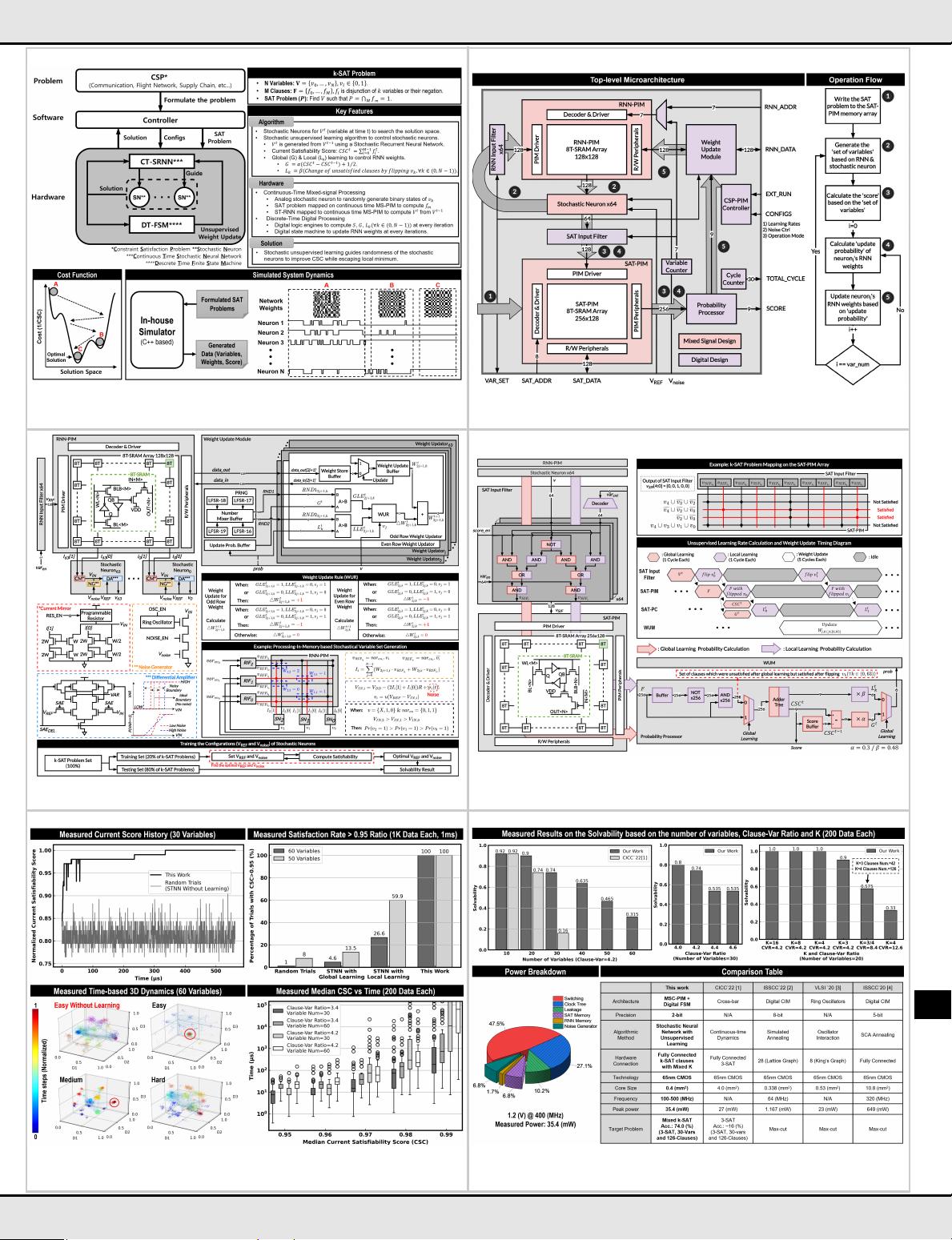
Figure 29.1.1 shows an overview of the proposed solver for a SAT problem (N variables
and M clauses). The variables (𝑣
𝑛
; ∀𝑛 ∈ (0,𝑁 − 1)) are represented by binary stochastic
neurons. A single layer fully connected recurrent neural network (RNN) uses a weighted
linear combination of past Boolean states of neurons to control a set of random
processes that determine neurons’ current states. The k-SAT (k≥3, each clause can have
different k) problems are programmed into a crossbar architecture to compute Boolean
states of the clauses (𝑓
𝑚
; ∀𝑚 ∈ (0,𝑀 − 1)). A digital FSM aggregates states of all clauses
to compute a current satisfiability score (CSC = the number of satisfied clauses) and
update the RNN weights to control the stochasticity of neurons. Updates to RNN weights
(2b integers) are governed by stochastic un-supervised global and local learning rules.
The temporal gradient of CSC is used to determine the probability of global learning (G)
for all RNN weights; a positive (negative) gradient increases (decreases) G. The
probability of local learning (L
k
) of weights connected to the k
th
neuron is determined by
flipping its state (𝑣
k
) and computing the change in the number of un-satisfied clauses; a
reduction in the number of unsatisfied clauses increases L
k
. The global and local learning
probabilities and current Boolean state of a neuron are used to update the weights
associated with that neuron. The global learning guides the system to evolve towards
higher CSC (global optima), while local learning helps escape from local minima. During
early iterations, neurons show high degree of stochasticity due to continuous changes
in the RNN weights (chaotic state). The weights and neurons converge to deterministic
states over iterations.
Figure 29.1.2 shows the system architecture and operation flow. Mixed-Signal
Processing-in-Memory (MS-PIM) modules implement the RNN (RNN-PIM) and the
crossbar for mapping/computing SAT clauses (SAT-PIM). The stochastic neurons are
realized using analog circuits with controllable randomness. Digital FSMs compute the
RNN weight update probabilities (Probability Processor, PR-PC) and use these
probabilities and a pseudo-random number generator (PRNG) to stochastically update
the RNN weights (Weight Update Module, WUM). A SAT input filter is used to connect
the neuron outputs to SAT-PIM and support the learning rules.
An SRAM array with 128 rows and 128 columns (2KB 8T-SRAM cells) implements the
RNN-PIM for 64 variables and 2b weights (Fig. 29.1.3). The weights are updated using
decoders and read/write peripherals connected to WL (column) and BL/BLB (row) of bit-
cells, respectively. The PIM operation is performed via IN and OUT terminals of the
bit-cell. The outputs from stochastic neurons (variable sets) are filtered using the RNN
Input Filter (RIF) to generate PIM inputs via SRAM rows. Each variable is associated with
two rows. The odd (2j+1) and even (2j) rows are associated with the true (𝑣
j
) and
complemented (𝑣
j
) forms of t he j
th
[∀𝑗 ∈ (0,63)] variable, respectively. RNN weights
𝑊
2j+1,k
and 𝑊
2j,k
represent influences of 𝑣
j
and 𝑣
j
(past states of j
th
variable) to the next
state of the k
th
variable (𝑣
k
), respectively. RIFs enable one (odd or even) row for each
variable (depending on the variable’s state) and disables both rows if a variable is not
included in a problem (an example is shown in Fig. 29.1.3). Vector matrix multiplication
(VMM) results are accumulated as current on the column lines. A pair of column lines
are connected to a stochastic neuron that includes a current mirror, noise generator and
a differential amplifier (Fig. 29.1.3). The current mirror for each neuron adds currents of
the corresponding column pair (with 2× gain for current of the MSB column) and
generates a membrane potential (V
IN
) for the neuron. A programmable noise generator
adds fluctuation to V
IN
. The differential amplifier determines the next Boolean state of
each variable by comparing the reference voltage with the noisy V
IN
. The added
programmable noise (controlled via V
REF
and V
noise
) and the inherent thermal noise of the
differential amplifier lead to stochastic neuron behavior.
The WUM consists of a PRNG and comparators (Fig. 29.1.3). The PRNG generates four
pseudo-random numbers (RNDs) using LFSRs and digitally mixes them to generate two
RNDs. A set of comparators, each connected to a row of RNN-PIM, generate global/local
learning enable (GLE/LLE) signals based on two RNDs and update probabilities. All
weights connected to one output neuron [i.e., for the k
th
neuron: 𝑊
2j+1,k
and 𝑊
2j,k
, ∀𝑗 ∈
(0,63)] are updated in parallel; weights for different neurons are updated in sequence.
For the k
th
neuron, the comparators generate 𝐺𝐿𝐸
2j+1,k
, 𝐿𝐿𝐸
2j+1,k
, 𝐺𝐿𝐸
2j,k
, and 𝐿𝐿𝐸
2j,k
,
which are coupled with 𝑣
k
to update (incremented by ‘1’, decremented by ‘1’, or remains
unchanged) 𝑊
2j+1,k
and 𝑊
2j,k
. The comparator reads, updates, and writes back the RNN
weights in 2, 1, and 2 cycles, respectively. The optimal configurations (V
REF
and V
noise
)
are decided by training (finding the optimal configuration). The optimal configurations
are different for each chip due to process variation.
Figure 29.1.4 shows the SAT input filter, SAT-PIM and the PR-PC for computing CSC
and weight update probabilities. Each row of a 256-row and 128-column SAT-PIM
(consists of 8T-SRAM cells) represents a clause. The columns represent variables 𝑣
k
and 𝑣
k
. The SAT problem is mapped by programming the bit-cells of the SAT-PIM to
indicate presence (‘1’) or absence (‘0’) of 𝑣
k
and 𝑣
k
in a clause (an example is shown in
Fig. 29.1.4). The SAT-PIM can map a maximum of 256 clauses, each with a maximum
of 64 variables; different clauses may also have different number of variables. All the
neuron states, expanded via SAT input filters to create 𝑣
k
and 𝑣
k
, are simultaneously
applied to the columns of SAT-PIM. All SRAM bit-lines (OUT in the bit-cell), representing
clauses, are pre-discharged. For each clause, any matching clause-input variable charges
the corresponding bit-line, indicating the clause is satisfied. The PR-PC accumulates the
clause outputs to compute CSC. The change in CSC between successive iterations is
used to compute G (Fig. 29.1.4). To support local learning, the PR-PC also stores the
set of unsatisfied clauses in an iteration. The SAT input filter inverts one variable (𝑣
k
) at
a time and the PR-PC determines corresponding L
k
by computing the change in the
number of unsatisfied clauses. L
k
values for all variables are computed in sequence.
Figure 29.1.5 shows measurement results from a prototype 65nm test chip operating at
1.2V, 400MHz, and at room temperature. A random search approach is also realized on
the chip by disabling PR-PC and WUM (no learning) as a baseline. The measured CSC
over time for a 30-variable and 126-clause 3-SAT problem shows the proposed method
achieves 100% CSC within 350μs, while the random search does not converge. The
probability of achieving 95% or higher CSC within 1ms is computed considering 1000
random 3-SAT problems. The random search shows 1% success for a 60-variable
252-clause problem compared to 100% success in the proposed method. Only using
global or local learning for the same problem shows 4.6% and 26.6% successes,
respectively. The evolution of variables over time is visualized using a T-distributed
stochastic neighbor embedding (t-SNE) to reduce a 60-dimensional (variable) space to
a 3-dimensional space; each marker represents a dimension-reduced variable-set and
the color represents the time-step. The random trials show chaotic search behavior even
for an easy (low clause to variable ratio) problem. The proposed approach shows fast
convergence to the optimum search area for easy problems, and harder (larger clause
to variable ratio) problems show more chaotic search behavior. The design demonstrates
99% satisfiability in 11.25ms and 125ms of median run-time for 3-SAT problems of 30
variables/126 clauses and 60 variables/252 clauses, respectively.
Figure 29.1.6 shows the measured data over 200 randomly generated k-SAT problems.
The solvability, defined as the percentage of these 200 cases where all clauses are
satisfied, reduces with an increasing number of variables and with a higher clause-to-
variable ratio (M/N). The measurement shows 74.0% solvability for 30 variables with
M/N=4.2, considered to be the hard region for 3-SAT. The design is flexible enough to
map and solve problems with higher k and mixed-k. The 0.4mm
2
core consumes 32.5mW
dominated by the clock and switching power of FSM. In comparison to a prior SAT solver,
the design shows smaller area, higher solvability for hard problems, and more flexibility
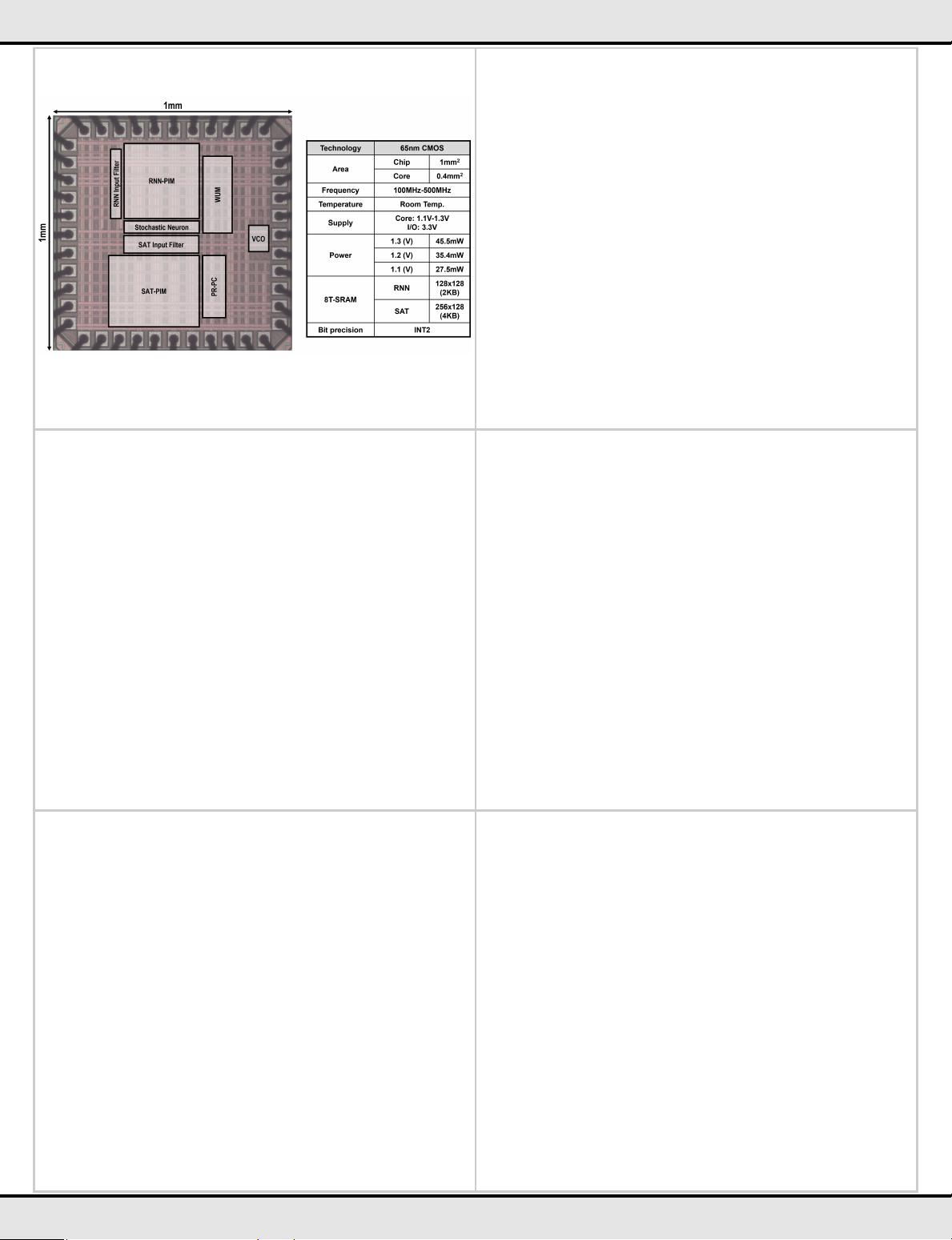
in mapping problems. Fig. 29.1.7 shows the die photo and the chip specifications.
References:
[1] M. Chang et al., “An Analog Clock-free Compute Fabric base on Continuous-Time
Dynamical System for Solving Combinatorial Optimization Problems,” IEEE CICC, 2022.
[2] Y. Su et al., “FlexSpin: A Scalable CMOS Ising Machine with 256 Flexible Spin
Processing Elements for Solving Complex Combinatorial Optimization Problems,” ISSCC,
pp. 274-275, 2022.
[3] I. Ahmed et al., “A Probabilistic Self-Annealing Compute Fabric Based on 560
Hexagonally Coupled Ring Oscillators for Solving Combinatorial Optimization Problems,”
IEEE Symp. VLSI Circuits, 2020.
[4] K. Yamamoto et al., “STATICA: A 512-Spin 0.25M-Weight Full-Digital Annealing
Processor with a Near-Memory All-Spin-Updates-at-Once Architecture for Combinatorial
Optimization with Complete Spin-Spin Interactions,” ISSCC, pp. 138-139, 2020.
978-1-6654-9016-0/23/$31.00 ©2023 IEEE