利用地下水-农艺耦合模型评价涝渍地区作物-土壤-水动态资源-CSDN文库

145 浏览量 2024-05-23 20:35:12 上传评论收藏 6.38MB PDF 举报

资源推荐

资源详情

资源评论

Environmental Modelling and Software 143 (2021) 105130

Available online 13 July 2021

Evaluating crop-soil-water dynamics in waterlogged areas using a coupled

groundwater-agronomic model

Chenda Deng

, Yao Zhang

, Ryan T. Bailey

Department of Civil and Environmental Engineering, Colorado State University, Fort Collins, CO, United States

Natural Resource Ecology Laboratory, Colorado State University, Fort Collins, CO, United States

ARTICLE INFO

Keywords:

Groundwater modeling

MODFLOW

DayCent

Message passing interface (MPI)

Waterlogging

Model coupling

ABSTRACT

Waterlogging on croplands has been a known problem for a long time, leading to adverse social, physical,

economic and environmental issues. To better solve the problem, the complicated plant-soil-water dynamics

system needs to be better understood. The challenge is to simulate the interactions between the components in

the systems. There are models that simulate plant-soil-water system but either run the processes independently

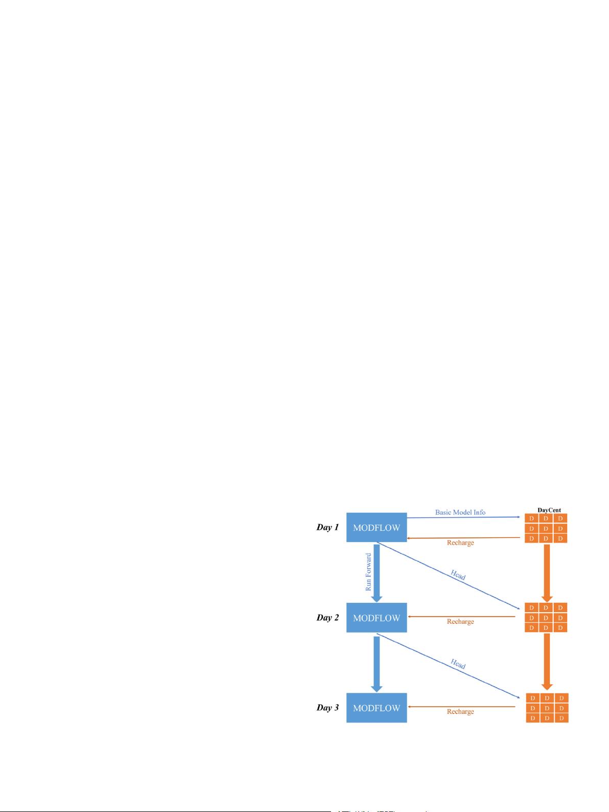
leading to inaccuracy or has high invasiveness of using integrated models. This paper presents a tightly coupled

model, DayCent-MODFLOW, that links a 3D ground-water ow (MODFLOW) model and a 1D agroecosystem

model (DayCent). DayCent is responsible for plant-soil-water dynamic in the root zone, whereas MODFLOW

simulates head and groundwater ow in the saturated zone of the aquifer. DayCent passes deep percolation from

the soil prole to the water table and, under conditions of waterlogging in which the water table is within the soil

prole, DayCent soil hydrologic processes are constrained by the presence of the water table simulated by

MODFLOW. The coupling is achieved by adopting a parallel inter-process communication technique MPI

(Message Passing Interface). The model is applied to a waterlogged agricultural area (22 km

) in northern

Colorado, USA and tested against groundwater head and rates of evapotranspiration (ET). The model runs in

parallel with multiple processes on the largest AWS Linux server. Groundwater heads match measured heads to a

reasonable degree, and ET rates match reference ET and are highly correlated with crop type. Results show the

strong hydrologic interaction between the two models. Greenhouse gas emissions from soil (N

O and CH

) were

also estimated by the model under the waterlogged conditions. Although the model can be used to simulate any

plant-soil-aquifer system, no matter the depth of the water table, results from this study show that the model can

be used to assess crop productivity, recharge, ET, and greenhouse gas emissions in areas of shallow groundwater.

1. Introduction

The plant-soil-water system controls the movement of water, nutri-

ents, and greenhouse gases in agricultural landscapes. Understanding

this system under a variety of hydrologic conditions is important for

food production, land management, water management, and nutrient

management. The plant-soil-water system is a complex system consist-

ing of surface water runoff, inltration, soil water dynamics, evapo-

transpiration, recharge and nutrient leaching, carbon (C)-nitrogen (N)

cycling, and consequent hydro-chemical processes such as ow and

nutrient transport in aquifers, stream discharge and nutrient loading,

and greenhouse gas emissions.

The challenge of simulating water transport and nutrient cycling in

such a complex system resides mainly in the interaction between

“zones”, such as water movement between the soil prole and the

saturated zone of the aquifer. As stated by Alley (Alley et al., 2002),

groundwater recharge is the most difcult groundwater budget to

simulate due to factors such as precipitation, irrigation application,

evapotranspiration, land use, crop type, and soil type. A special condi-

tion of plant-soil-water interaction is the presence of saturated condi-

tions in the root zone of crops (i.e. “waterlogging”), which can decrease

crop yield and damage soil health and structure (Cannell et al., 1980;

Cavazza and Pisa, 1988; Collaku & Harrison, n.d.; Houk et al., 2006,

2006, 2006; Kaur et al., 2017). $360 million loss of crop production

every year during 2010–2016 is due to waterlogging and even greater

loss than drought in the United States (Ploschuk et al., 2018). Water-

logging can dramatically change the dynamics of carbon and nitrogen in

soil. The resulting anaerobic condition decreases the rate of organic

* Corresponding author.

E-mail address: cddpeter@rams.colostate.edu (C. Deng).

Contents lists available at ScienceDirect

Environmental Modelling and Software

journal homepage: www.elsevier.com/locate/envsoft

https://doi.org/10.1016/j.envsoft.2021.105130

Accepted 3 July 2021

Environmental Modelling and Software 143 (2021) 105130

matter decomposition (Meurant and Riker, 2014), resulting in an

accumulation of soil organic matter that affects nitrogen mineralization

and available nitrogen for crop uptake; and also increases denitrica-

tion, which can increase methane (CH

) emission and nitrous oxide

O) emission (Bartlett and Harriss, 1993; Parton et al., 2001), both of

which are greenhouse gases.

There are many numerical physically based models that simulate a

range of hydrologic and chemical processes in the plant-water-soil sys-

tem. A subset of these models is agronomic models that simulate hy-

drologic in a one-dimensional domain at the soil prole-scale. These

include SWAP (Kroes et al., 2009), DSSAT (Jones et al., 2003), and

DayCent (Parton et al., 1998; Zhang et al., 2018a,b). They simulate

irrigation, runoff, inltration, and percolation through soil layers, crop

ET, and deep percolation from the bottom of the soil prole. However, as

they do not simulate groundwater ow in the saturated zone of the

underlying aquifer, the uctuation of the water table and its possible

presence in the soil prole and crop root zone is not represented. The

Soil & Water Assessment Tool (SWAT) (Arnold et al., 1998) simulates

hydrological processes and crop yield at the watershed scale, with a

water balance occurring at individual hydrologic response units (HRUs)

across the watershed landscape. The model accounts for groundwater

storage and groundwater discharge to streams but does not simulate

water table uctuation in a physically based manner and hence cannot

account for waterlogging effects on root zone processes and crop yield.

Even the linked SWAT-MODFLOW model (Bailey et al., 2016) does not

account for the condition of shallow groundwater in the root zone –

MODFLOW may simulate a water table at the elevation of an HRU’s soil

prole, but it has no effect on SWAT’s HRU soil prole and root zone

processes. The linked DSSAT-MODFLOW model (Xiang et al., 2020) also

does not account for the effect of shallow groundwater on root zone

processes, as the linkage between the models is performed at the annual

time scale, and day-to-day DSSAT root zone hydrological processes are

not affected by MODFLOW-simulated water table elevation.

Another subset of models simulates vadose zone hydrologic pro-

cesses and water table uctuation, but do not simulate near-surface

hydrology, vegetative growth, root zone processes, and nutrient

cycling. These include the hydrologic and hydrogeologic models MOD-

FLOW (Niswonger et al., 2011), HYDRUS (

Simůnek et al., 2012),

MODFLOW-SURFACT (Panday and Huyakorn, 2008), STOMP (White

and Oostrom, 2003), TOUGH2 (Pruess et al., 1999), VS2DI (Healy,

2008), the VSF package (Thoms et al., 2006), and HydroGeoSphere

(Therrien et al., 2010), among many others. There is a general lack of

hydro-agronomic models wherein the simulated water table affects root

zone processes, and root zone processes in turn affect recharge to the

water table.

The objective of this paper is to present a coupled agroecosystem-

groundwater modeling system that can simulate water movement

under waterlogged conditions. The DayCent and MODFLOW are chosen

as the agroecosystem and groundwater models, respectively. DayCent

was selected as it includes carbon and nitrogen dynamics in agro-

ecocystems, and thus is more versatile in applications. MODFLOW is

chosen as it is the most widely used groundwater ow model worldwide

(Langevin et al., 2017). The models are tightly coupled, with system

data passed between them on a daily time step, using a novel Message

Passing Interface (MPI) (Gropp et al., 1996) that avoids code modi-

cation to DayCent and MODFLOW codes and therefore can work with

updated versions of DayCent and MODFLOW. DayCent improves

recharge calculations to MODFLOW, and MODFLOW improves the ac-

curacy of crop yield and nutrient cycling of DayCent in the presence of a

shallow water table. Although the DayCent-MODFLOW linked system

can be applied to any plant-soil-water system, an application to an

irrigated area with shallow groundwater in northern Colorado, USA, will

be shown to demonstrate its capability in waterlogged conditions. The

impact of waterlogged conditions on greenhouse gases will also be

briey described in the model application.

2. Methods

This section provides information about the DayCent and MODFLOW

models and a description of how they are tightly coupled using the MPI

method.

2.1. Introduction to MODFLOW: groundwater ow model

MODFLOW is Fortran-written program (Koelbel et al., 1994) that

numerically solves the three-dimensional ground-water ow equation

by using a nite-difference method (McDonald and Harbaugh, 1988;

Niswonger et al., 2011). MODFLOW is the most widely used ground-

water ow model in the world. Versions include MODFLOW-88

(McDonald and Harbaugh, 1988), MODFLOW-96 (Harbaugh and

McDonald, 1996), MODFLOW-2000 (Harbaugh et al., 2000),

MODFLOW-NWT (Niswonger et al., 2011) and MODFLOW-6 (Langevin

et al., 2017). In this study, MODFLOW-NWT version is used to couple

with DayCent due to its efciency and focus on solving nonlinear

systems.

MODFLOW-NWT simulates groundwater head throughout an aquifer

system by solving the groundwater ow equation for a porous medium.

The ow equation for an unconned aquifer (Bedekar et al., 2012) is:

∂

) +

∂

) +

∂

(f (F)K

∂

) + W = ϕ

∂

+ F

∂

(1)

where x, y, z are the three dimensions; h is groundwater head (L); K is

hydraulic conductivity (L/T). S

is specic storage (1/T). ϕis porosity

taken equal to specic yield S

; F

is the fraction of the cell thickness that

is saturated; and f(F) is a function of F

set to 1 for Niswonger et al.

(2011).

MODFLOW also solves the equation for conned aquifers, but this

study is concerned with water table interaction in soil zones, and hence

Equation (1) is presented. The nite difference method is used to solve

Equation (1) by discretizing the groundwater system spatially into a grid

of cells and the simulation time period into time steps. Each cell is

interpreted as a small volume of aquifer material with the same hy-

draulic properties. The equation describes the volumetric water balance

within each of the cell, with groundwater inputs including groundwater

ow from adjacent cells and other groundwater sources (e.g., recharge,

seepage) and groundwater outputs including ow to adjacent cells and

other groundwater sinks (e.g. ET, pumping, discharge). The aquifer

hydraulic properties include hydraulic conductivity K, specic yield S

and specic storage S

. Although the primary variable of solution is

groundwater head h, ow rates using h can be calculated at each time

step.

2.2. Introduction to DayCent: agroecosystem model

The DayCent model (William J. Parton et al., 1998; Zhang et al.,

2018) is a medium complexity agroecosystem model. The major

sub-models of DayCent are plant growth, soil water, soil organic carbon,

soil nitrogen and Greenhouse gas uxes. Major inputs for the model are

daily weather, soil physical properties, plant type, and management

practices. DayCent has been widely used for carbon and nitrogen sim-

ulations in agroecosystems (S. J. Del Grosso et al., 2008; Stephen J. Del

Grosso et al., 2006; Robertson et al., 2018; Zhang et al., 2013). The

model was selected to estimate soil CO

and N

O emissions/removals for

the US national greenhouse gas inventory (USEPA, 2021) which is

annually submitted to the UN Framework Convention on Climate

Change (United Nations, 1992). The crop growth/production sub-model

has been used in simulations of agroecosystem dynamics not only in the

U.S. but also globally (Cheng et al., 2014; S. J. Del Grosso et al., 2008;

Gautam et al., 2020; Lee et al., 2012; Stehfest et al., 2007; Zhang et al.,

2020). Recently, the DayCent model has been improved in simulations

of crop canopy development, growth, and water use (Zhang et al., 2020;

C. Deng et al.

Environmental Modelling and Software 143 (2021) 105130

Zhang et al., 2018; Zhang et al., 2018). This new version of DayCent is

used in this study for coupling with MODFLOW. DayCent is written in

Fortran and C (Kernighan and Ritchie, 2006).

The DayCent modeling code includes the main water balance com-

ponents for a soil prole: inltration of precipitation and irrigation,

surface runoff, deep percolation from the bottom of the soil prole,

evapotranspiration (ET; evaporation and transpiration), and capillary

rise of groundwater:

ΔS

= P + I

net

− ET

− RO − DP + GW (3)

where ΔS

is the net change in soil water at the end of day i and i-1. In this

equation, P, RO, and DP are precipitation, runoff, and deep percolation

on day i, respectively. I

net

is the net irrigation on day i. GW is the ground

water contribution if a shallow water table is present. ET

is the actual

evapotranspiration on day i. All units are in cm day-1. The soil prole is

dened by users which is usually less than 3 m in depth. The input soil

parameters include soil texture, bulk density, and eld capacity, wilting

point, and saturated hydraulic conductivity.

Reference ET is simulated using either the standardized Penman-

Monteith method (Allen et al., 1998) or the Hargreave’s method (Har-

greaves and Allen, 2003), with the latter used when only air temperature

is available. The solar radiation, wind speed, and relative humidity are

required to run the Penman-Monteith method. Crop coefcients are used

in conjunction with reference ET to estimate potential ET for each crop

type. The ET is partitioned into potential evaporation and potential

transpiration as a function of the green canopy coverage and residue

coverage. The green canopy coverage (CC) is calculated from Beer’s law

(Monsi and Saeki, 1953; SELLERS, 1985):

CC = 1 − exp( − k × GLAI) (4)

where k (dimensionless) is the light extinction coefcient of the vege-

tation, and GLAI is green leaf area index (m m-1). The GLAI and CC

approach was recently added to DayCent and the detailed description

can be found in Zhang et al. (2018a,b). Water uptake by root is limited

by soil available water. Regarding potential soil evaporation, it can be

reduced by the amount of standing dead biomass and litter on the soil

surface. In DayCent, actual evaporation is also limited by the soil water

potential of the top soil layer and the upward uxes from underlying

layers (Parton et al., 1998).

DayCent simulates 1D water ows using a combined method: a

modied tipping-bucket approach for water ow above eld capacity

and a Richards’ approach (Richards, 1931) for water re-distribution

below eld capacity (Parton et al., 1998). Water table is simply simu-

lated by turning off the drainage of water at the last soil layer for a

user-specied period. When water table is present, the water inltrated

from soil surface starts to saturate soil from the bottom. In the linked

DayCent-MODFLOW, the presence of water table in DayCent simulation

is controlled by the water table elevation in MODFLOW (Section 2.3).

Nitrogen dynamics are simulated in DayCent model using the mass

balance of nitrogen in soil:

ΔN = N

littter

+ N

fert

+ N

deposit

− N

gas

− N

erosion

− N

Root

(5a)

where N

litter

is nitrogen added from plant litter; N

fert

includes both

organic and inorganic fertilizer; N

deposit

is atmospheric nitrogen depo-

sition; N

gas

is gas removed via nitrication and denitrication and in-

cludes N

, N

O, and NO

gases; N

erosion

is the loss due to soil erosion; N

is the removal from the soil prole via deep percolation (both inorganic

and organic forms); and N

Root

is plant root upake.

The emission of CH

is produced in soil under anaerobic conditions

by methanogens. In DayCent, the rate is primarily determined by the

availability of carbon substrate (derived from decomposition and root

rhizo-deposition) for methanogens and the impact of environmental

variables including soil texture (redox potential, pH, and soil tempera-

ture), climate, and agricultural practices (Hartmann et al., 2016).

Methane oxidation under aerated conditions is also modeled by DayCent

as a function of soil temperature, soil water content, porosity, and eld

capacity (Grosso et al., 2000) (Del Grosso et al., 2000). DayCent simu-

lates soil N

O and NO

emissions from nitrication and denitrication

(W. J. Parton et al., 2001). Nitrication is calculated as a function of soil

ammonium (NH

) concentration, soil moisture, soil temperature, pH,

and soil texture. Denitrication is a function of soil nitrate concentra-

tion, labile carbon availability, O

availability, soil water content, and

soil physical properties that inuence gas diffusivity.

2.3. Description of DayCent-MODFLOW theory

This section describes the basic linkage between DayCent and

MODFLOW, i.e. which information is passed between the two models,

and when. Section 2.4 provides details regarding the Message Passing

Interface (MPI) used to link the models without invasive code modi-

cation to either DayCent or MODFLOW. Section 2.5 describes an

application of DayCent-MODFLOW to a waterlogged site in an agricul-

tural area of northern Colorado, USA.

DayCent-MODFLOW is linked on a daily time step, with results from

each model providing inputs and constraints on the other. Therefore, the

linkage could be termed “tight linkage” or “tight coupling”. The linkage

process through time steps of a simulation is shown in Fig. 1. Each

DayCent model is mapped to one cell of the top layer of the MODFLOW

grid. As DayCent is a 1D eld-scale model, multiple DayCent simulations

are included to represent the collection of cultivated elds overlying the

unconned aquifer. Therefore, multiple DayCent models are linked to a

single MODFLOW model based on the geological locations. The simu-

lation runs according to the following steps, repeated for each time step:

1. MODFLOW passes basic grid cell information to the set of DayCent

models: surface elevation (top of MODFLOW grid cells), bottom

elevation of MODFLOW grid cells, specic yield S

of aquifer mate-

rial, and saturated hydraulic conductivity K of top layer (Table 1).

The soil and aquifer properties are shared between DayCent and

MODFLOW. If the time step is the rst of the simulation, MODFLOW

also passes initial groundwater head values for each grid cell.

2. The received values are assigned to corresponding model variables

for each DayCent model.

3. Each DayCent model is run for the time step.

Fig. 1. Flow chart of data passing in the coupled DayCent-MODFLOW model,

showing a single MODFLOW model coupled with a set of eld-based Day-

Cent models.

C. Deng et al.

剩余11页未读，继续阅读

评论收藏

内容反馈

___Y1

粉丝: 5148
资源: 160

利用地下水-农艺耦合模型评价涝渍地区作物-土壤-水动态

论文研究 - 农艺性能和感官评价Lablab（

学习软件_早教启蒙_乐乐英语--农艺园 1.0免费下载.zip

论文研究-黑龙港地区棉花栽培综合农艺措施数学模型的研究.pdf

论文研究 - 氮肥和水分管理方式对水稻的农艺，水分生产率和经济性分析

节水灌溉理论与技术教（学）案.doc

论文研究- 农作物栽培技术系统决策模型库及其应用.pdf

论文研究 - 水稻的农艺和生理响应

行业资料-交通装置-一种园林农艺用手推车.zip

利用花生染色体片段置换系群体评价部分农艺性状及与SSR标记的相关性

8个紫花苜蓿品种在山西中部地区的农艺性状和营养价值评价.pdf

论文研究 - 利用诱变育种高粱：纳米比亚的未来前景

农艺高级工考试题-11页.pdf

论文研究 - 模拟气候变化对玉米的影响（

大数据-算法-油菜高产优质栽培综合农艺措施的数学模型及优化方案.pdf

论文研究 - 马达加斯加南部15个向日葵基因型农艺性能和种子油成分的评估

论文研究 - 改进的补充灌溉对干旱地区农场收入，生产效率和风险管理的影响

孟加拉国模拟玉米生长和产量的农业技术转让模型决策支持系统的校准和验证

重点研发计划项目申报指南.doc

基于Android的可定制作物育种数据采集系统设计与实现.pdf

Origin绘制相关性热图插件(Correlation Plot)

（免费）Chrome浏览器插件axure-chrome-extension

vep视频快速加密提取器

糖尿病数据集diabetes.csv（免费）

最新版YS9082HC主控开卡工具 YS9082HC-MPToolV8.00.00.18.826-HCS1A25E2023062

2011-2022年北大数字普惠金融指数数据（包括省市县）.zip

2024春 四川农业大学 数字电子技术 期末机考试卷答案

noc指导教师资格认证题库

IEEE 802.11be（WiFi7） 协议原文pdf文档

ESRI-Licensing文件夹，安装arcgispro无法破解登录

最新资源

2024春四川农业大学数字电子技术期末机考试卷答案

IEEE 802.11be（WiFi7）协议原文pdf文档