
Scalable Deep Gaussian Markov Random Fields for General Graphs
GMRFs with Convolutional Neural Networks (CNNs) for
the special case of image-structured data. DGMRFs can be
trained efficiently and keep all useful properties of GMRFs,
such as exact Bayesian inference for the latent field. In this
paper we extend and generalize the DGMRF framework
to the general graph setting. This requires us to design a
new layer construct for DGMRFs based on local operations
over node neighborhoods. Without making any assumptions
on the graph structure we propose methods that allow the
model training to scale to massive graphs.
Our main contributions are: 1) We extend the DGMRF
framework to general graphs by designing a new type of
layer construct based on GNNs. 2) We adapt the DGMRF
training to this new setting, making use of an improved
variational distribution. 3) We propose scalable methods
for performing the log-determinant computations central to
the training. 4) We demonstrate properties of the resulting
model on synthetic data. 5) We experiment on multiple real-
world datasets, for which our model outperforms existing
methods.
2. Background
2.1. GMRFs
In graphical models a set of random variables are associ-
ated with the nodes of a graph (Koller & Friedman, 2009;
Bishop, 2006). GMRFs are undirected graphical models
where the nodes jointly follow a Gaussian distribution. More
specifically, let
G
be an undirected graph with
N
nodes
concatenated in the random vector
x ∈ R
N
. We say that
x ∼ N
µ, Q
−1
is a GMRF with mean
µ
and precision ma-
trix
Q
w.r.t. the graph
G
iff
Q
i,j
6= 0 ⇔ j ∈ n(i), ∀i 6= j
,
where
n(i)
is the exclusive neighborhood of node
i
(
i /∈
n(i)
). A GMRF is thus a multivariate Gaussian with a pre-
cision matrix as sparse as the graph. Note however that the
covariance matrix can still be fully dense, enabling depen-
dencies between all nodes in the graph.
Consider now the common situation where we observe
y = x +
,
∼ N
0, σ
2
I
. A GMRF prior on
x
is conju-
gate to this Gaussian likelihood. We will mainly consider
the application of GMRFs to problems where
y
is observed
only for some nodes. Let
m ∈ {0, 1}
N
be a mask vector
with ones in positions corresponding to the observed nodes,
y
m
= y m
and
I
m
= diag(m)
. The posterior for
x
in
this setting is then given by x|y
m
∼ N
˜
µ,
˜
Q
−1
, where
˜
Q = Q +
1
σ
2
I
m
(1a)
˜
µ =
˜
Q
−1
Qµ +
1
σ
2
y
m
. (1b)
While the posterior is analytically tractable, and again a
GMRF, computing the involved entities explicitly can be a
significant computational challenge for large N.
2.2. DGMRFs
Sid
´
en & Lindsten (2020) note that for an affine map
g: R
N
→ R
N
a GMRF x can be defined by
z = g(x) = Gx + b, z ∼ N(0, I) (2)
where
G ∈ R
N×N
is a matrix and
b
some offset vector. This
results in a GMRF with mean
µ = −G
−1
b
and precision
matrix
Q = G
|
G
. Note how the direction of the mapping
in Eq. 2 makes
x
implicitly defined, a different setup from
other generative models mapping Gaussian noise to data.
The affine map
g
can in turn be defined as a combination of
L
simpler layers as
g = g
(L)
◦ g
(L−1)
◦ ··· ◦ g
(1)
, adding
the depth to the Deep GMRF. The value of considering the
layers separately is that they can be implemented implicitly,
using some operation that is known to be affine. Thus,
multiple such operations can be chained without performing
the expensive matrix multiplications to create G.
Sid
´
en & Lindsten (2020) consider the special case where
the entries of
x
are associated with pixels in an image. They
then define each
g
(l)
as a 2-dimensional convolution with
a filter containing trainable parameters. Such a DGMRF
is a GMRF w.r.t. a lattice graph (Rue & Held, 2005), a
graph where each pixel is connected to neighboring pixels
within a window determined by the filter size. The resulting
model shares much of its structure with CNNs. This allows
for utilizing existing deep learning frameworks for efficient
convolution computations, automatic differentiation, and
GPU support.
After observing some data
y
m
inference for the latent field
x
follows from Eq. 1. To avoid inverting
˜
Q
, the posterior
mean
˜
µ
can be computed using the Conjugate Gradient
(CG) method (Hestenes & Stiefel, 1952; Shewchuk, 1994).
Often, also the posterior marginal variances
Var[x
i
|y
m
]
are of interest. To avoid computing the covariance matrix
explicitly, an alternative is to use a Monte Carlo estimate
based on a set of samples from the posterior. It is possible
to use the CG method also for efficiently drawing posterior
samples (Papandreou & Yuille, 2010).
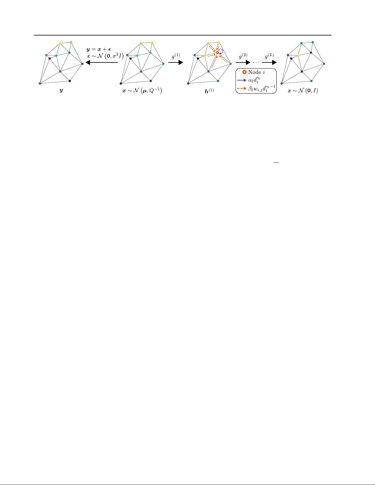
3. DGMRFs on Graphs
We extend the DGMRF framework of Sid
´
en & Lindsten
(2020) to general graphs, removing the assumption of a
lattice graph to match the general definition of a GMRF.
To achieve this we design a new type of layer
g
(l)
without
any assumptions on the graph structure. We then propose
a way to train this new type of DGMRF using scalable
log-determinant computations and a new, more flexible,
variational distribution. An overview of our model is shown
in Figure 2.


评论0
最新资源