Wireless Sensor Networking in Matlab:
Step-by-Step
Milan Simek, Patrik Moravek and Jorge sa Silva
Abstract—We present an extensive guide for the researchers
that aim to validate proposed algorithms for wireless sensor
networks in Matlab environment. In this paper, we describe step
by step all necessary tasks that must be accomplished for the
full operation of the Matlab WSN simulation model. The goal of
this paper is to describe processes how to simulate the lifetime
of the WSN network during a data gathering. We describe tasks
such as topology generation and visualization, data routing and
communication cost calculation. To estimate lifetime of network,
we have proposed the Matlab energy model that goes from the
analysis of the real Zigbe network.
Index Terms—wireless sensor networks, Matlab, implementa-
tion, simulation, guide, matrix.
I. INTRODUCTION
T
HIS paper introduces step-by-step implementation of
the wireless sensor networking in Matlab environ-
ment(particularly Matlab 2007b). It aims to bring detailed
directions for under/postgraduate students and researches deal-
ing with the wireless sensor simulation under the Matlab
environment. Hence a longterm data gathering is the funda-
mental task of the wireless sensor networks, we show how to
implement all necessary tasks related with the data gathering
processes. In the considered simulation, each battery equipped
node unicasts in the regular intervals (refferred to as rounds of
data gathering) a one packet with the defined size. The packets
are multihoped through the network to the base station that
is power supplied. Simulation ends when there is no path to
the base station, meaning that all neighbors of base station
are out of energy. The results of the simulation are presented
by the colored topology showing the residual energy on each
node and a plot of number of alive nodes in the network
during increasing number of gathering rounds. The rest of
paper is structured as follows: Section I brings the steps of
network topology definition. In Section II, we show how to
find the shortest path between two nodes in ad-hoc network.
An evaluation of communication cost is introduced in Section
III, while Section IV describes the proposed energy model.
The result of the entire simulation are presented in Section V.
The section VI brings the conclusion and future work.
II. NETWORK TOPOLOGY
A network with N nodes can be modeled as a N -vertex
undirected graph G = (V = {1, ..., N}, E), where 2D/3D
Manuscript received December 15, 2010; revised January 11, 2010.
M. Simek and Patrik Moravek are with the Department of Telecom-
munication of Brno University of Technology, Czech Republic, e-
mail:simek@feec.vutbr.cz
Jorge sa Silva is with Department of Informatics, University of Coimbra,
Portugal, email:sasilva@dei.uc.pt.
position p of each vertice i is identified by the set of coordi-
nates p
i
= (x
i
, y
i
and z
i
respective). An euclidean length d
i,j
between two vertices i, j ∈ V is refferred to as E. The network
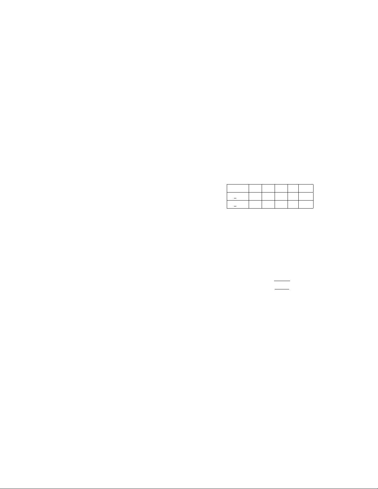
topology is then interpreted by a three/four row matrix, where
the 2D/3D position of nodes are stored in individual columns,
see Table I. Furthermore for a simplicity, only the 2D plane
is considered for the simulation.
TABLE I
TOPOLOGY MATRIX
ID 1 2 3 ... N
X coor x
1
x
2
x
3
... x
N
Y coor y
1
y
2
y
3
... y
N
For the simulations, the networks are considered to be fully
connected, meaning that all nodes are reachable due to the
multihop communication. The connectivity depends on the
radio range, thus the radio range of the nodes should be
configured optimally. One can estimate the optimal radio range
empirically or to use an Eq. 1 that estimates the minimum
radio range ensuring the full connectivity.
R = Θ
r
log N
N
(1)
The Θ parameter stands for a 2D plane diameter directly
proportional to the number of nodes N. Calculating the R
for the 100 nodes randomly placed in the 2D plane with the
300m x 500m dimension, the minimal R should be 82 meters.
According to the experiences with the Crossbow IRIS 2.4
GHz node [7], the radio range of 82 meters corresponds to
the transmitting power of 3.2 dBm.
Once the network matrix is created and radio range calcu-
lated, the network topology can be printed. The layout of the
network consists of the vertices and edges between vertices.
The edge or link between two nodes can be printed only in
case that the euclidean distance d
i,j
between two nodes i, j
is smaller than R of the considered nodes. Since the wireless
links are considered to be bidirectional and symmetric then
d
i,j
= d
j,i
. A pseudocode of the layout printing is introduced
in more details in the following section.
In the real wireless network, a distance between two nodes
can be derived from RSSI parameter (Receive Signal Strength
Indication) or estimated by methods such as ToA (Time of
Arrival) or AoA (Angle of Arrival) [11]. These techniques
suffer from the certain distance estimation error and thus this
error should be also implemented into the simulation model.