


SYSC-4600
Lab 1
Digital Bandpass Transmission
Department of Systems and Computer Engineering Page 2 of 14
1 Purpose and Objectives
The purpose of this laboratory experiment is to provide familiarity with some of
the more popular digital passband transmission systems.
The influence of the transmitter and/or the receiver filtering operations on the
received signal are examined both in the time-domain, and in the frequency
domain. The lab provides some insight into the differences between two of the
popular Modulation methods: Binary Phase Shift Keying (BPSK), Quadrature
Phase Shift Keying (QPSK).
Impact of receiver filtering on the received signal is also examined with emphasis
on qualitative effect on ISI. The construction of matched filters and their impact
on the received signal are also examined.
Please note that this lab is designed more as a tutorial to provide students with a
visual, hands on insight into the many basic concepts of passband transmission.
You are encouraged to invent ways of using it on your own.
2 Background
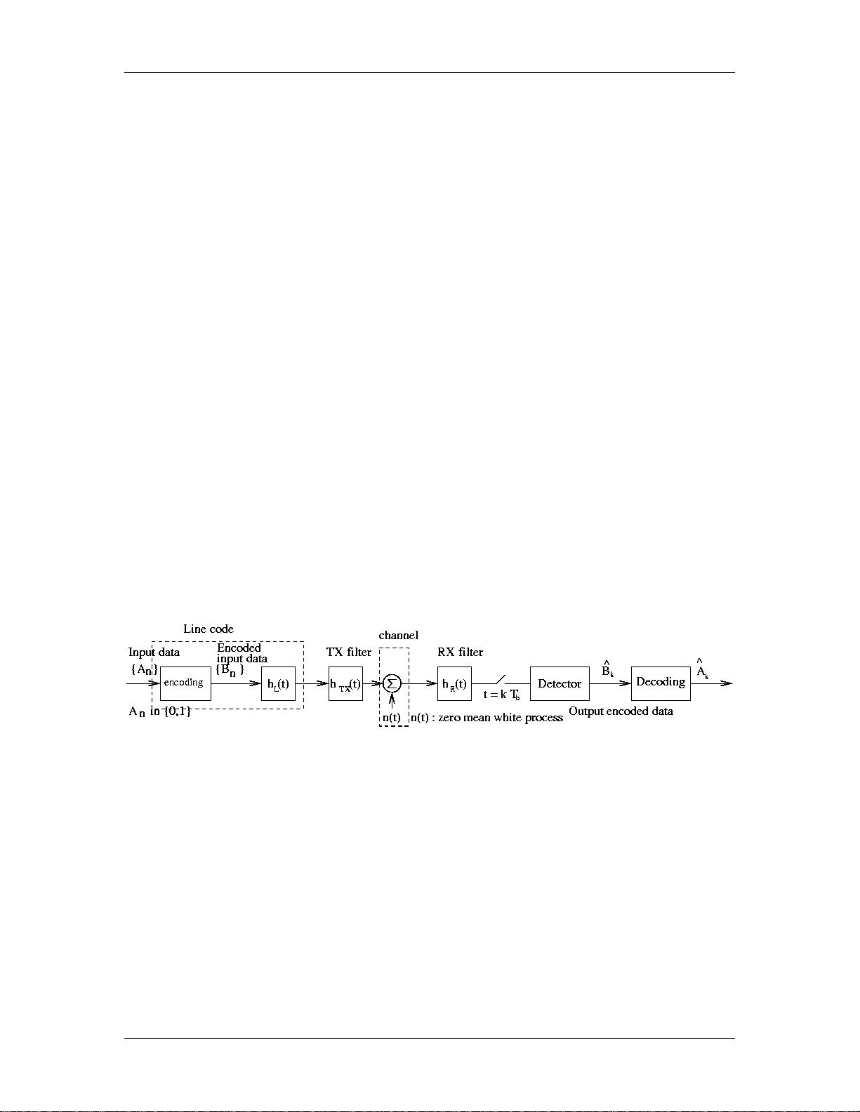
A simplified block diagram of a passband BPSK communication system is shown
in Fig.1 (will be changed):
Figure 1: Simplified block diagram of a passband BPSK communication system
The bit stream {A
n
} (sequence of ‘0’ and ‘1’) could have been generated from a
digital information, from the character coding of textual information (ex. Think
being represented as the bit stream 001010 | 000100 | 100100 | 011100 |
110100) or from the sampling, quantization and encoding of an analog source.
The bit stream is then pulse modulated to generate an antipodal binary
baseband pulse waveform, i.e. a ‘1’ is represented by a pulse p(t) and a ‘0’ is
SYSC4600 – Digital Communication Laboratory #2

Department of Systems and Computer Engineering Page 3 of 14
represented by a pulse –p(t). The pulse shape p(t)
1
will vary according to the
line code used, and depends on any filters in the transmitter, i.e. p(t) = h
L
(t) *
h
TX
(t), where h
L
(t) is the filter of the line code and h
TX
(t) is the transmit filter(TX)
impulse response. The baseband pulse waveform is multiplied by a sinusoidal
carrier to generate a BPSK modulated signal. A coherent demodulator extracts
the data by first down converting the BPSK signal to baseband. The baseband
signal is applied to a receive filter. The receive filter output is applied to a
decision device. The receiver filter response could be that of a simple lowpass
filter with a given cut-off frequency. It could also be a “matched filter”. The
matched filter response is a time-reversed replica of the transmitter pulse shape
p(t). In this lab, a matched filter will be used, i.e. h
R
(t) = p(T
b
–t). In Fig. 1, an
AWGN channel with an infinite bandwidth has been assumed (i.e., excluding the
additive noise, the channel impulse response is h
c
(t)=δ(t)).
It is convenient for analysis and simulation to consider the line code filter and the
TX filter as one filter, called the transmitter filter, with impulse response h
T
(t)
given by h
T
(t) = h
L
(t) * h
TX
(t) as illustrated in Fig.2.
Figure 2: Simplified block diagram of a passband communication system (line
code pulse shaping + TX filtering combined into one block) (will be changed)
This section will be updated to include background on optimal detection in AWGN
noise.
***************************************************************
Part I of this laboratory will consider the effect of the choice of line codes
2
and
the TX filter
3
on the power spectral density of the transmitted signal v(t)
4
.
Looking at Fig.3, we see that the transmitted signal is passed through an AWGN
channel with an infinite bandwidth (i.e., h
c
(t)=δ(t), or equivalently no filter h
c
(t)
1
For implementation purposes it is often convenient to synthesize the transmitter pulse shape p(t) using a
single block. This is the approach used in this lab.
2
i.e., effect of encoding and h
L
(t)
3
i.e., effect of h
TX
(t)
4
signal coming out of the filter h
T
(t)
SYSC4600 – Digital Communication Laboratory #2

Department of Systems and Computer Engineering Page 4 of 14
is present in the channel model). The received signal (after transmission over the
channel) is then passed through a receiver filter h
R
(t). The receiver filter impulse
response could be that of a simple lowpass filter with a given cut-off frequency.
It could also be a “matched filter”. The matched filter impulse response is a time-
reversed replica of the transmitter pulse shape h
T
(t) (i.e., h
R
(t) = h
T
(T
b
-t))
Let us assume that a polar NRZ line code with a rectangular pulse shape time-
limited from 0 to T
b
is used in a baseband communication system with no TX
filtering (i.e., h
TX
(t) =δ(t), h
T
(t)=rect( (t- T
b
/2) /T
b
) ), over an ideal noiseless
channel that has an infinite bandwidth (i.e., no n(t) present and h
c
(t) =δ(t)), and
assume no filtering at the receiver (i.e., h
R
(t) =δ(t)), then the output of the
receiver filter y(t) to one bit (let us say A
0
=1) equals B
0
h
T
(t)= h
T
(t) and hence
spans in time from 0 to T
b
. When a sequence of bits is transmitted, then the
output to the second bit will span in time from T
b
to 2T
b
, and thus will not
interfere with the output to the first bit. Therefore in that case there is no
Intersymbol Interference (ISI), and a decision can be made on B
0
or equivalently
on A
0
by sampling the output of the receiver filter at any time between 0 and
T
b
. Furthermore, because the channel was assumed to be noiseless, no decision
error will be made.
In practice, the channel introduces some additive noise, and therefore the
receiver includes a receiver filter before sampling to improve performance. The
purpose of the receiver filter is to filter part of the noise to reduce the number of
decision errors. As shown in the lecture notes, the filter that will maximize the
signal-to-noise ratio at the output of the receiver filter at a given sampling time
(and hence will reduce the number of decision errors over an AWGN channel) is
the matched filter, i.e, a filter with impulse response h
R
(t) = h
T
(T
b
–t) assuming a
sampling time equal to T
b.
A second effect will occur involving the principle of duality between time and
frequency, namely absolutely time-limited waveforms cannot be absolutely band-
limited and absolutely band-limited waveforms cannot be absolutely time-limited.
In practice, the channel will have a finite bandwidth; therefore the transmitter
will have to include filters to ensure that the bandwidth of the transmitted signal
after filtering is smaller than the channel bandwidth. Due to the duality between
time and frequency, considering a transmitter filter of finite bandwidth means
that the filter impulse response has infinite time duration. Practically, H
T
(f) will
be almost band-limited and h
T
(t) will be almost time-limited, but of duration that
may span more than one bit duration (more than Tb). This means that the
output to one bit will span from 0 to more than Tb, and thus will interfere with
the output to the second bit of the transmitted sequence. In other words ISI will
occur. In that case, the output of the receiver filter at the sampling time used to
detect B
0
is composed of a term proportional to B
0
, a noise term and a term that
represents the contribution of the past bits, called ISI. The value of the ISI term
SYSC4600 – Digital Communication Laboratory #2

Department of Systems and Computer Engineering Page 5 of 14
will depend on h
c
(t) if the channel has a finite bandwidth, the choice of h
T
(t) and
h
R
(t), the choice of sampling time as well as the values of the past transmitted
bits. Note that in a system model it is also possible to include all the filtering
effect of the channel in the transmitter filter h
T
(t) and assume for simplicity that
h
c
(t) = δ(t), this approach is considered in this lab. If the composite pulse shape
h(t) = h
T
(t) * h
c
(t) * h
R
(t) (here = h
T
(t) * h
R
(t)) satisfies Nyquist criterion, like
root raised cosine or sinc pulse shapes for example, then the ISI term equals to
zero. Note that this requires to know the channel impulse response exactly, so in
practice even though h
T
(t) and h
R
(t) are designed so that Nyquist criterion is
satisfied, there is always some residual ISI due to the imperfect estimation of the
channel impulse response. In one example in this lab, h
T
(t) and h
R
(t) will be
squared root raised cosine pulse shapes yielding a root raised cosine composite
pulse h(t) = h
T
(t) * h
R
(t).
Choice of sampling time:
Let us assume that it is known that A
0
=1 (or equivalently B
0
=1 for polar NRZ)
was transmitted, then the best sampling time would the one such that the value
of the output of the receiver filter at the sampling time (including the ISI and
noise term) is the closest to 1, in other words is maximum. Let us assume that it
is known that A
0
=0 (or equivalently B
0
=-1 for polar NRZ) was transmitted, then
the best sampling time would the one such that the value of the output of the
receiver filter at the sampling time (including the ISI and noise term) is the
closest to -1, in other words is minimum. Of course in practice, the value of A
0
is not known beforehand, so the sampling time should be chosen taking into
account all possible cases. Since the ISI term depends on past transmitted bits,
all possible transmitted sequences should be considered. The eye diagram is a
convenient way to find the best sampling time as well as how sensitive a
communication system is to noise given a choice of transmitter filter and receiver
filter. The eye diagram at the output of the receiver filter is obtained by plotting
on the same graph the output of the receiver filter assuming all possible
combination of transmitted bits (i.e., all possible transmitted sequences). Using
this method, the obtained graph will display for example the output of the
receiver filter when A
0
=1 and when A
0
=-1 (assuming all possible sequences of
past bits). By looking at the eye diagram, the best sampling time that will be
suitable for both cases can be deduced. Usually the best sampling time is at a
point where the eye is opened at the widest, thus yielding the output of the
receiver filter closer to 1 for the curve corresponding to A
0
=1, or closest to –1 for
the curve corresponding to A
0
=-1.
A typical eye diagram is as follows:
SYSC4600 – Digital Communication Laboratory #2


