


UNIVERSITY OF
NEWCASTLE UPON TYNE
School of Electrical, Electronic and Computer
Engineering
Matlab/Simulink Tutorial
Release 13 - version 6.5
Second Edition
June 2003

Contents
CHAPTER 1: The Basics ......................................................................................... 1
1.1 Introduction ................................................................................................................1
1.2 Simple math............................................................................................................... 2
1.3 Matlab and variables.................................................................................................. 2
1.4 Variables and simple math ........................................................................................ 4
1.5 Complex numbers...................................................................................................... 4
1.6 Common mathematical functions .............................................................................. 5
1.7 M-files ........................................................................................................................ 6
1.8 Workspace................................................................................................................. 8
1.9 Number display formats............................................................................................. 8
1.10 Path Browser ........................................................................................................... 8
1.11 Toolboxes. ............................................................................................................... 8
1.12 Help………............................................................................................................... 8
CHAPTER 2: Arrays and Plots................................................................................ 9
2.1 Array construction...................................................................................................... 9
2.2 Plots ........................................................................................................................... 9
2.3 Array addressing...................................................................................................... 12
2.4 Array Construction ................................................................................................... 14
2.5 Array Orientation...................................................................................................... 16
2.6 Array – Scalar Mathematics .................................................................................... 17
2.7 Array-Array mathematics ......................................................................................... 18
2.8 Zeros, Ones, … ....................................................................................................... 19
2.9 Array Manipulation................................................................................................... 20
2.10 Array Searching and Comparison ......................................................................... 21
2.11 Array Size .............................................................................................................. 22
2.12 Matrix operations ................................................................................................... 23
CHAPTER 3: Strings, Logic and Control Flow..................................................... 25
3.1 Strings...................................................................................................................... 25
3.2 Relational and Logical Operations........................................................................... 25
3.2.1 Relational Operators............................................................................................... 25
3.2.2 Logical Operators.................................................................................................... 26
3.3 Control flow.............................................................................................................. 27
3.3.1 “for” loops................................................................................................................ 27
3.3.2 “while” Loops........................................................................................................... 28
3.3.3 if-else-end Constructions ........................................................................................ 29
CHAPTER 4: Polynomials, Integration & Differentiation .................................... 30
4.1 Polynomials ............................................................................................................. 30
4.2 Numerical Integration............................................................................................... 32
4.3 Numerical Differentiation ......................................................................................... 33
4.4 Functions ................................................................................................................. 34
4.4.1 Rules and Properties .............................................................................................. 34
CHAPTER 5: Introduction to Simulink ................................................................. 36
5.1 Introduction .............................................................................................................. 36
5.2 Solving ODE ............................................................................................................ 36
5.2.1 Example 1............................................................................................................... 39
5.2.2 Example 2............................................................................................................... 43
5.2.3 Example 3............................................................................................................... 45
5.2.4 Exercise ..................................................................................................................45
5.3 Second Order System Example .............................................................................. 46
5.4 Fourier Spectrum Example ...................................................................................... 53
UNIVERSITY OF NEWCASTLE UPON TYNE
SCHOOL OF ELECTRICAL, ELECTRONIC AND COMPUTER ENGINEERING
MATLAB BASICS – SECOND EDITION
Chapter 1 Page 1
CHAPTER 1: The Basics
1.1 Introduction
Matlab stands for Matrix Laboratory. The very first version of Matlab, written at the University of
New Mexico and Stanford University in the late 1970s was intended for use in Matrix theory, Linear
algebra and Numerical analysis. Later and with the addition of several toolboxes the capabilities of
Matlab were expanded and today it is a very powerful tool at the hands of an engineer.
Typical uses include:
• Math and Computation
• Algorithm development
• Modelling, simulation and prototyping
• Data analysis, exploration and visualisation
• Scientific and engineering graphics
• Application development, including graphical user interface building.
Matlab is an interactive system whose basic data element is an ARRAY. Perhaps the easiest way
to visualise Matlab is to think it as a full-featured calculator. Like a basic calculator, it does simple
math like addition, subtraction, multiplication and division. Like a scientific calculator it handles
square roots, complex numbers, logarithms and trigonometric operations such as sine, cosine and
tangent. Like a programmable calculator, it can be used to store and retrieve data; you can create,
execute and save sequence of commands, also you can make comparisons and control the order
in which the commands are executed. And finally as a powerful calculator it allows you to perform
matrix algebra, to manipulate polynomials and to plot data.
To run Matlab you can either double click on the appropriate icon on the desktop or from the start
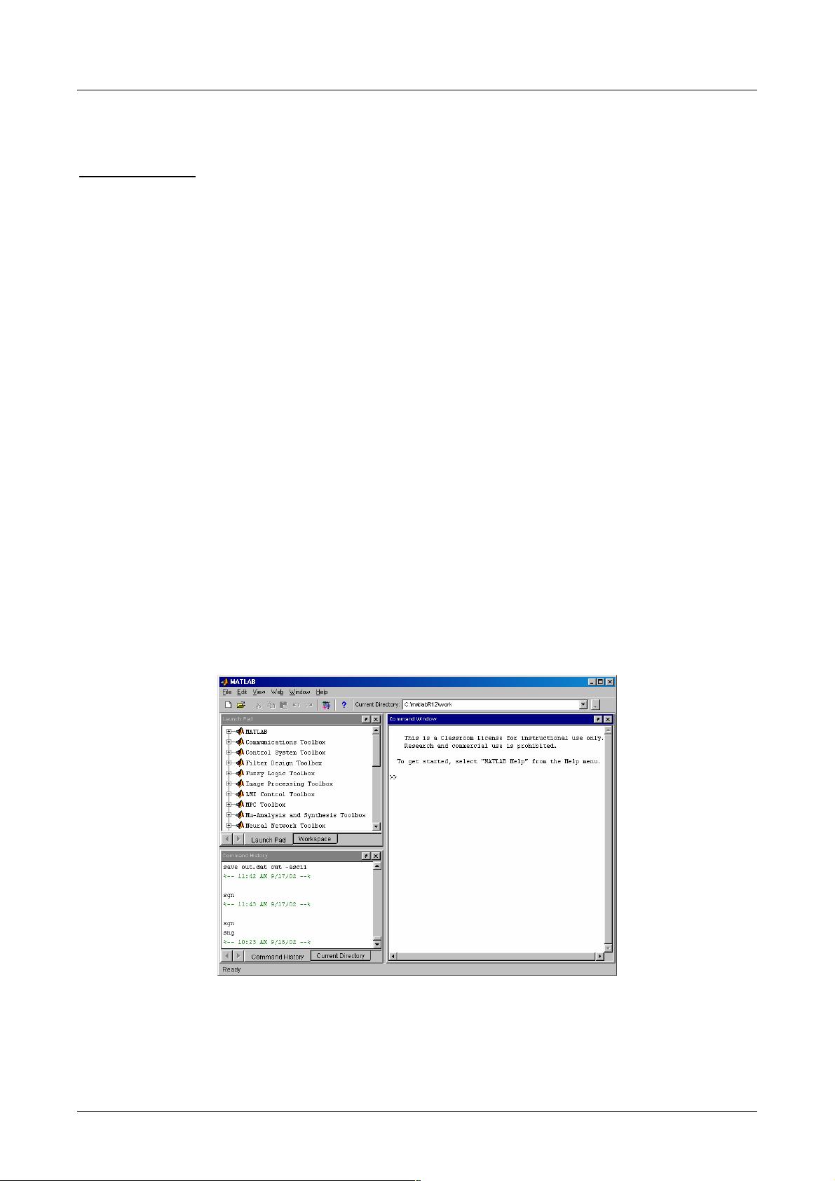
up menu. When you start Matlab the following window will appear:
Figure 1: Desktop Environment
Initially close all windows except the “Command window”. At the end of these sessions type
“Demo” and choose the demo “Desktop Overview” for a full description of all windows. The
command window starts automatically with the symbol “>>” In other versions of Matlab this symbol
may be different like the educational version: “EDU>>”. When we type a command we press
ENTER to execute it.

UNIVERSITY OF NEWCASTLE UPON TYNE
SCHOOL OF ELECTRICAL, ELECTRONIC AND COMPUTER ENGINEERING
MATLAB BASICS – SECOND EDITION
Chapter 1 Page 2
1.2 Simple math
The first thing that someone can do at the command window is simple mathematic calculations:
» 1+1
ans =
2
» 5-6
ans =
-1
» 7/8
ans =
0.8750
» 9*2
ans =
18
The arithmetic operations that we can do are:
Operation Symbol Example
Addition, a+b + 5+3
Subtraction, a-b - 5.05-3.111
Multiplication, a*b * 0.124*3.14
Left division, a\b \ 5\3
Right division, b/a / 3/5(=5\3)
Exponentiation, a
b
^ 5^2
The order of this operations follows the usual rules: Expressions are evaluated from left to right,
with exponentiation operation having the highest order of precedence, followed by both
multiplication and division, followed by both addition and subtraction. The order can change with
the use of parenthesis.
1.3 Matlab and variables
Even though those calculations are very important they are not very useful if the outcomes cannot
be stored and then reused. We can store the outcome of a calculation into variables by using the
symbol “=”:
» a=5
a=
5
UNIVERSITY OF NEWCASTLE UPON TYNE
SCHOOL OF ELECTRICAL, ELECTRONIC AND COMPUTER ENGINEERING
MATLAB BASICS – SECOND EDITION
Chapter 1 Page 3
» b=6
b=
6
» newcastle=7
newcastle =
7
» elec_elec_sch=1
elec_elec_sch =
1
We can use any name for our variables but there are some rules:
• The maximum numbers of characters that can be used are 63
• Variable names are case sensitive, thus the variable “A” is different from “a”.
• Variable names must start with a letter and they may contain letters, numbers and
underscores but NO spaces.
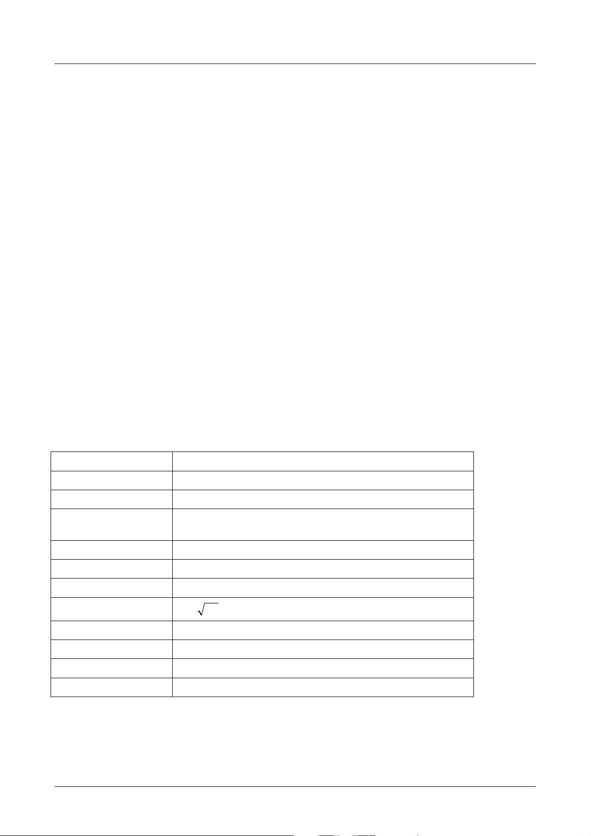
Also at the start of Matlab some variables have a value so that we can use them easily. Those
values can be changed but it is not wise to do it. Those variables are:
Special variable Value
ans The default variable name used for results
pi 3.14…
eps The smallest possible number such that, when added to
one, creates a number greater than one on the computer
flops Count of floating point operations. (Not used in ver. 6)
inf Stands for infinity (e.g.: 1/0)
NaN Not a number (e.g: 0/0)
I (and) j
i=j=
1−
nargin Number of function input arguments used
nargout Number of function output arguments used
realmin The smallest usable positive real number
realmax The largest usable positive real number
Also there are names that you cannot use: for, end, if, function, return, elseif, case, otherwise,
switch, continue, else, try, catch, global, persistent, break.
If we want to see what variables we have used, we use the command “who”:


评论0