4-机器学习系列(4):提高深度网络性能之 - 优化算法及python实现1
需积分: 0 169 浏览量
2022-08-03
11:48:24
上传
评论
收藏 1.99MB PDF 举报

机器学习系列(4)
提高深度网络性能之 - 优化算法
深度学习中反向传播的目标是,找到最优的参数(如W、b),使得代价函数(cost function)最小,如何使得代价函数更好收敛以及如何加快收敛过
程,分别对应着深度网络对精度和速度的要求,那么好的优化算法就显得至关重要了,一个好的优化算法能够大大提高整个团队的效率。本次将讨论反
向传播中的优化算法。
优化算法:
梯度下降
mini-bacth梯度下降
随机梯度下降
动量梯度下降
RMSprop
Adam
学习率衰减
Adamw
Python实现:
见文章内容
申明
本文原理解释及公式推导部分均由LSayhi完成,供学习参考,可传播;代码实现部分的框架由Coursera提供,由LSayhi完成,详细数据及代码可在
github查阅。
https://github.com/LSayhi/DeepLearning (https://github.com/LSayhi/DeepLearning)
微信公众号:AI有点可ai
优化算法
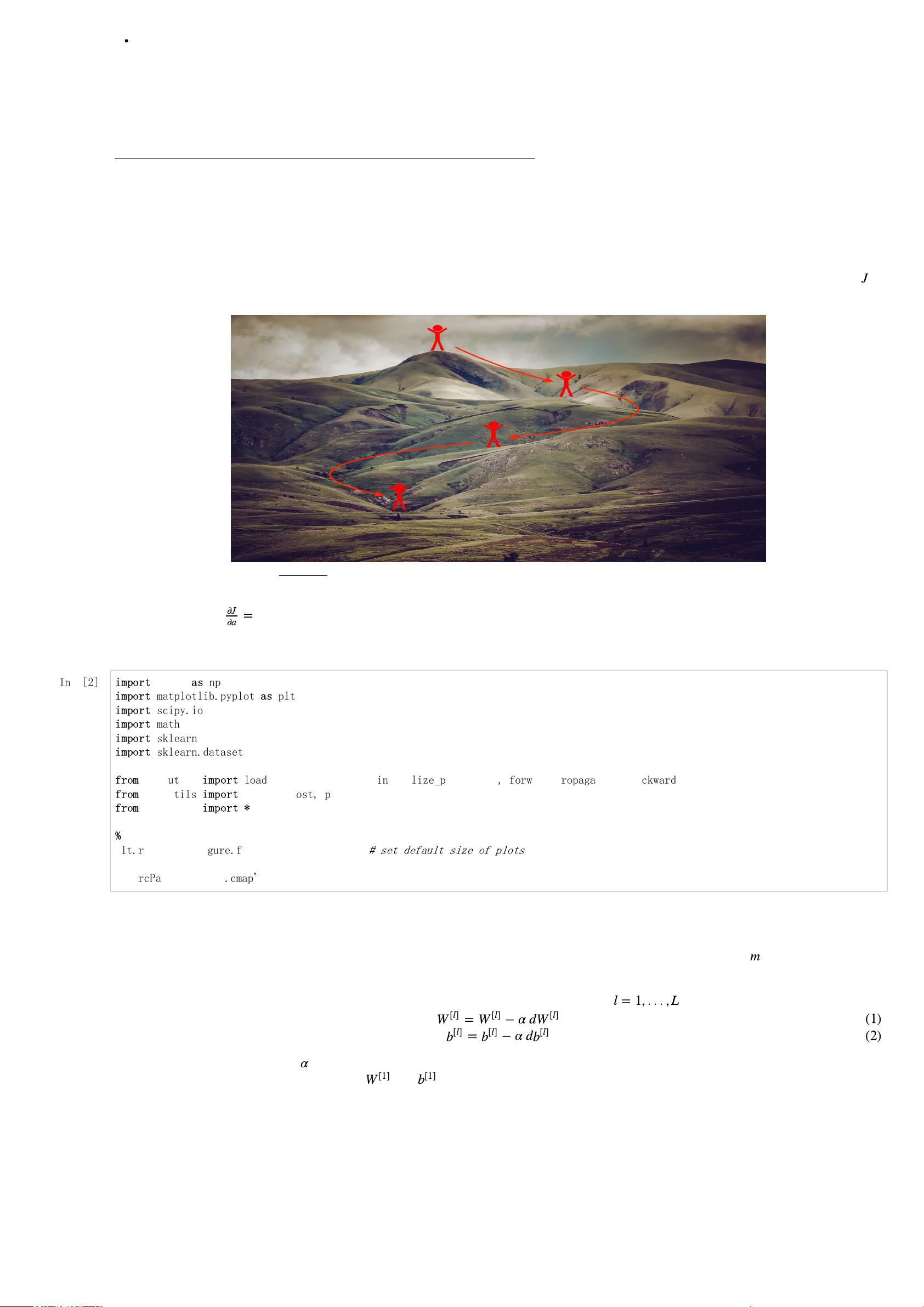
一、Bacth梯度下降
Bacth梯度下降指的是批量梯度下降(Batch Gradient Descent),是在寻找最优参数W和b的过程中,我们使用凸优化理论中的梯度下降方式,而
且每一步操作都是对整个训练集(所有m个样本)一起操作的。批量梯度下降算法,for l = 1, ..., L:
这里的L指的是网络层数,lpha指的是学习率(learning_rate).
批量体现在,将所有m个样本向量化,这样就可以避免使用显式for循环,从而降低时间复杂度,这样做的好处是能够大大减小梯度下降所需的的时
间,很可能原本需要几天的过程,现在只需几个小时。
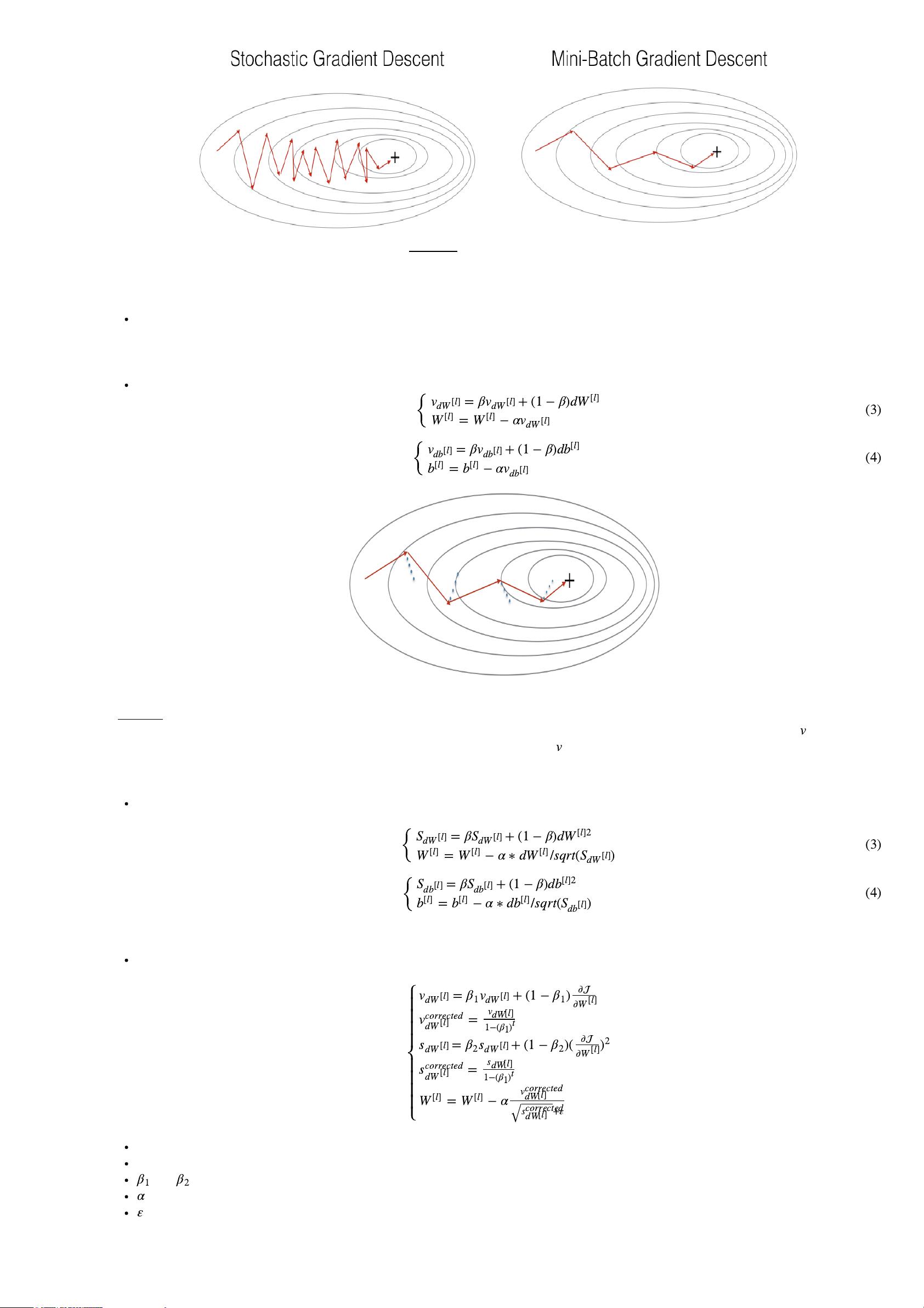
二、Mini-bacth 梯度下降
Mini-bacth梯度下降是指将所有m个样本分为多个小集合(每个小集合就称为mini-bacth),然后再分别应用梯度下降法,这样做的原因是,虽然批
量梯度下降法已经通过向量化大大减小了训练时间,但是当训练集的数目很大的话,处理速度仍然很慢,因为你必须每次处理所有的训练样本,然
后更新参数,再不断迭代。Mini-bacth梯度下降把m个样本分成了很多子训练集,先处理一个子集,更新参数,然后再处理一个子集,再更新参数,
这样会让算法速度更快。
mini-bacth梯度下降速度比bacth梯度下降更快,但由于不是对整个训练集进行操作,最优化的过程“摆动性”更强,会在cost function会在最小值附近
摆动。
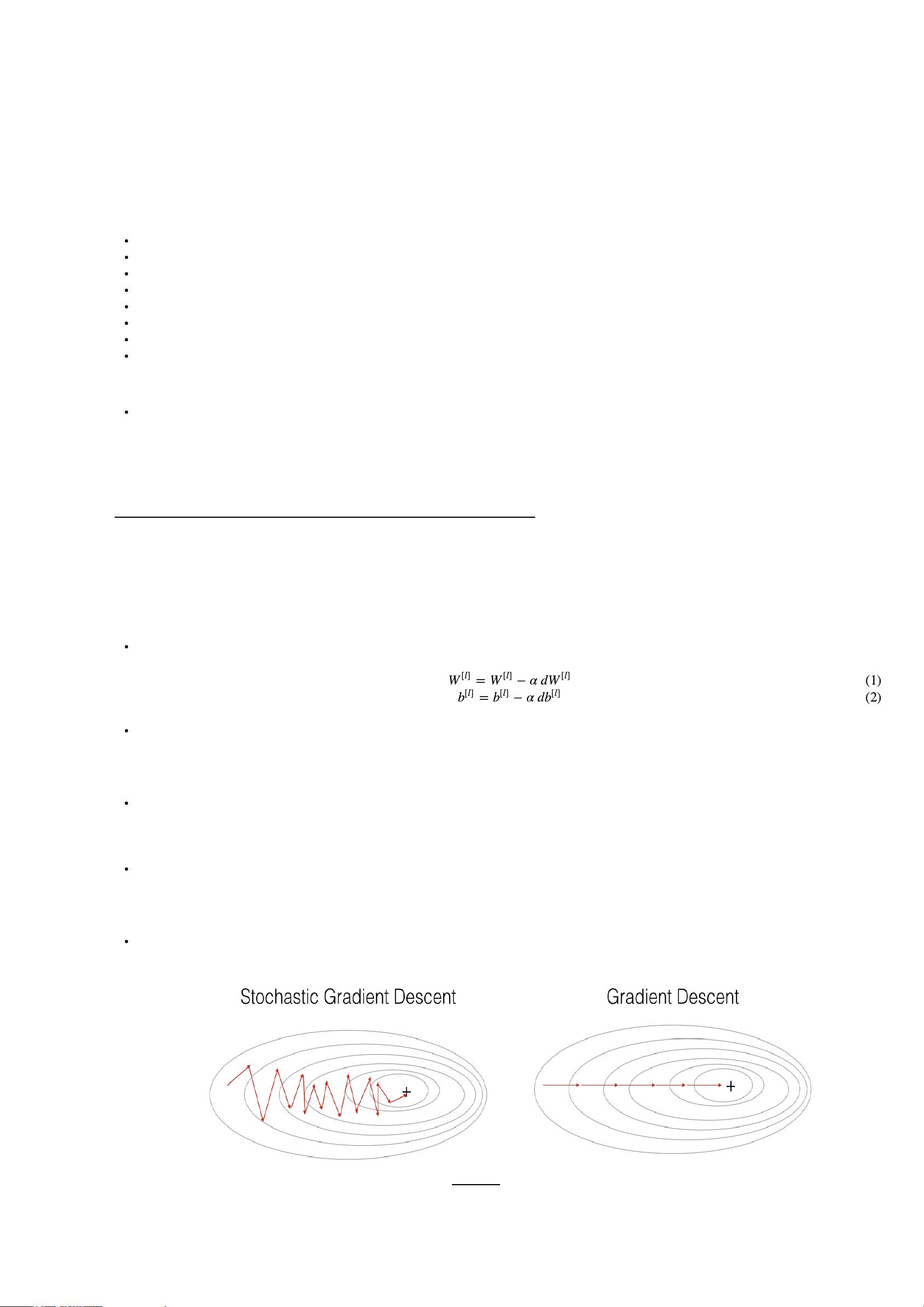
三、Stochastic梯度下降
Stochastic梯度下降即随机梯度下降,随机梯度下降可以看作是mini-batch的大小为1,这种方式最优化过程摆动性比mini-batch还要强,但是优点是
速度会比mini-batch还要快。
Figure 1 : SGD vs GD
"+" denotes a minimum of the cost. SGD leads to many oscillations to reach convergence. But each step is a lot faster to compute for SGD than
for GD, as it uses only one training example (vs. the whole batch for GD).
=
−
α
d
W
[
l
]
W
[
l
]
W
[
l
]
(1)
=
−
α
d
b
[
l
]
b
[
l
]
b
[
l
]
(2)
剩余19页未读,继续阅读
资源评论


