5
any ground-truth box. Note that a single ground-truth
box may assign positive labels to multiple anchors.
Usually the second condition is sufficient to determine
the positive samples; but we still adopt the first
condition for the reason that in some rare cases the
second condition may find no positive sample. We
assign a negative label to a non-positive anchor if its
IoU ratio is lower than 0.3 for all ground-truth boxes.
Anchors that are neither positive nor negative do not
contribute to the training objective.
With these definitions, we minimize an objective
function following the multi-task loss in Fast R-CNN
[2]. Our loss function for an image is defined as:
L({p
i
}, {t
i
}) =
1
N
cls
X
i
L
cls
(p
i
, p
∗
i
)
+λ
1
N
reg
X
i
p
∗
i
L
reg
(t
i
, t
∗
i
).
(1)
Here, i is the index of an anchor in a mini-batch and
p
i
is the predicted probability of anchor i being an
object. The ground-truth label p
∗
i
is 1 if the anchor
is positive, and is 0 if the anchor is negative. t
i
is a
vector representing the 4 parameterized coordinates
of the predicted bounding box, and t
∗
i
is that of the
ground-truth box associated with a positive anchor.
The classification loss L
cls
is log loss over two classes
(object vs. not object). For the regression loss, we use
L
reg
(t
i
, t
∗
i
) = R(t
i
− t
∗
i
) where R is the robust loss
function (smooth L
1
) defined in [2]. The term p
∗
i
L
reg
means the regression loss is activated only for positive
anchors (p
∗
i
= 1) and is disabled otherwise (p
∗
i
= 0).
The outputs of the cls and reg layers consist of {p
i
}
and {t
i
} respectively.
The two terms are normalized by N
cls
and N
reg
and weighted by a balancing parameter λ. In our
current implementation (as in the released code), the
cls term in Eqn.(1) is normalized by the mini-batch
size (i.e., N
cls
= 256) and the reg term is normalized
by the number of anchor locations (i.e., N
reg
∼ 2, 400).
By default we set λ = 10, and thus both cls and
reg terms are roughly equally weighted. We show
by experiments that the results are insensitive to the
values of λ in a wide range (Table 9). We also note
that the normalization as above is not required and
could be simplified.
For bounding box regression, we adopt the param-
eterizations of the 4 coordinates following [5]:
t
x
= (x − x
a
)/w
a
, t
y
= (y − y
a
)/h
a
,
t
w
= log(w/w
a
), t
h
= log(h/h
a
),
t
∗
x
= (x
∗
− x
a
)/w
a
, t
∗
y
= (y
∗
− y
a
)/h
a
,
t
∗
w
= log(w
∗
/w
a
), t
∗
h
= log(h
∗
/h
a
),
(2)
where x, y, w, and h denote the box’s center coordi-
nates and its width and height. Variables x, x
a
, and
x
∗
are for the predicted box, anchor box, and ground-
truth box respectively (likewise for y, w, h). This can
be thought of as bounding-box regression from an
anchor box to a nearby ground-truth box.
Nevertheless, our method achieves bounding-box
regression by a different manner from previous RoI-
based (Region of Interest) methods [1], [2]. In [1],
[2], bounding-box regression is performed on features
pooled from arbitrarily sized RoIs, and the regression
weights are shared by all region sizes. In our formula-
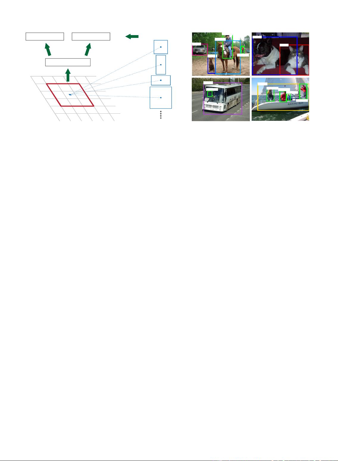
tion, the features used for regression are of the same
spatial size (3 × 3) on the feature maps. To account
for varying sizes, a set of k bounding-box regressors
are learned. Each regressor is responsible for one scale
and one aspect ratio, and the k regressors do not share
weights. As such, it is still possible to predict boxes of
various sizes even though the features are of a fixed
size/scale, thanks to the design of anchors.
3.1.3 Training RPNs
The RPN can be trained end-to-end by back-
propagation and stochastic gradient descent (SGD)
[35]. We follow the “image-centric” sampling strategy
from [2] to train this network. Each mini-batch arises
from a single image that contains many positive and
negative example anchors. It is possible to optimize
for the loss functions of all anchors, but this will
bias towards negative samples as they are dominate.
Instead, we randomly sample 256 anchors in an image
to compute the loss function of a mini-batch, where
the sampled positive and negative anchors have a
ratio of up to 1:1. If there are fewer than 128 positive
samples in an image, we pad the mini-batch with
negative ones.
We randomly initialize all new layers by drawing
weights from a zero-mean Gaussian distribution with
standard deviation 0.01. All other layers (i.e., the
shared convolutional layers) are initialized by pre-
training a model for ImageNet classification [36], as
is standard practice [5]. We tune all layers of the
ZF net, and conv3 1 and up for the VGG net to
conserve memory [2]. We use a learning rate of 0.001
for 60k mini-batches, and 0.0001 for the next 20k
mini-batches on the PASCAL VOC dataset. We use a
momentum of 0.9 and a weight decay of 0.0005 [37].
Our implementation uses Caffe [38].
3.2 Sharing Features for RPN and Fast R-CNN
Thus far we have described how to train a network
for region proposal generation, without considering
the region-based object detection CNN that will utilize
these proposals. For the detection network, we adopt
Fast R-CNN [2]. Next we describe algorithms that
learn a unified network composed of RPN and Fast
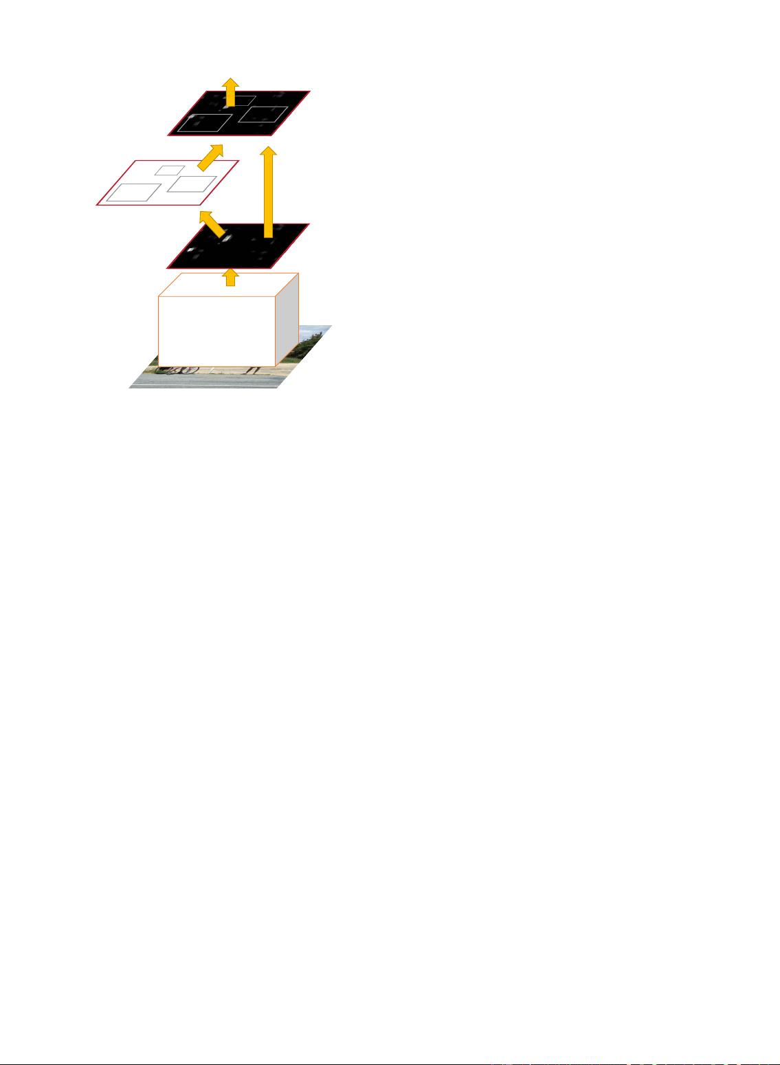
R-CNN with shared convolutional layers (Figure 2).
Both RPN and Fast R-CNN, trained independently,
will modify their convolutional layers in different
ways. We therefore need to develop a technique that
allows for sharing convolutional layers between the

 Faster R-CNN .rar (1个子文件)
  Faster R-CNN .pdf 6.59MB

 我的内容管理
展开
 我的资源
快来上传第一个资源
 我的收益 登录查看自己的收益
 我的积分
登录查看自己的积分
 我的C币
登录后查看C币余额
 我的收藏
我的收藏  我的下载
我的下载  下载帮助
下载帮助 
 前往需求广场,查看用户热搜

 信息提交成功
