没有合适的资源?快使用搜索试试~ 我知道了~
SPC document 质量统计控制 英文版
需积分: 10 17 下载量 25 浏览量
2016-02-22
16:01:47
上传
评论
收藏 626KB PDF 举报
温馨提示
试读
23页
This technical note on statistical quality control (SQC) covers the quantitative aspects of quality management. In general, SQC is a number of different techniques designed to evaluate quality from a conformance view. That is, how well are we doing at meeting the specifications that have been set during the design of the parts or services that we are providing? Managing quality performance using SQC techniques usually involves periodic sampling of a process and analysis of these data using statistically derived performance criteria.
资源推荐
资源详情
资源评论
T ECHNICAL N OTE S EVEN
technical note
Assignable variation defined 300
Common variation defined
Variation around Us 301
Upper and lower specification or tolerance limits defined
Process Capability 302
Capability index (C
pk
) Capability index (C
pk
) defined
Process Control Procedures 305
Process control with attribute Statistical process control (SPC) defined
measurements: using p charts Attributes defined
Process control with variable measurements: Variables defined
using X
–
and R charts
How to construct X
–
and R charts
Acceptance Sampling 311
Design of a single sampling plan for attributes
Operating characteristic curves
Conclusion 314
technical note seven
PROCESS CAPABILITY AND
STATISTICAL QUALITY
CONTROL
cha06369_tn07.qxd 2/12/03 7:01 PM Page 299
This technical note on statistical quality control (SQC) covers the quantitative aspects of
quality management. In general, SQC is a number of different techniques designed to
evaluate quality from a conformance view. That is, how well are we doing at meeting the
specifications that have been set during the design of the parts or services that we are pro-
viding? Managing quality performance using SQC techniques usually involves periodic
sampling of a process and analysis of these data using statistically derived performance
criteria.
As you will see, SQC can be applied to both manufacturing and service processes. Here
are some examples of the types of situations where SQC can be applied:
• How many paint defects are there in the finish of a car? Have we improved our paint-
ing process by installating a new sprayer?
• How long does it take to execute market orders in our Web-based trading system?
Has the installation of a new server improved the service? Does the performance of
the system vary over the trading day?
• How well are we able to maintain the dimensional tolerance on our three-inch ball
bearing assembly? Given the variability of our process for making this ball bearing,
how many defects would we expect to produce per million bearings that we make?
• How long does it take for customers to be served from our drive-through window
during the busy lunch period?
Processes that provide goods and services usually exhibit some variation in their output.
This variation can be caused by many factors, some of which we can control and others that
are inherent in the process. Variation that is caused by factors that can be clearly identified
and possibly even managed is called assignable variation. For example, variation caused by
workers not being equally trained or by improper machine adjustment is assignable varia-
tion. Variation that is inherent in the process itself is called common variation. Common
variation is often referred to as random variation and may be the result of the type of equip-
ment used to complete a process, for example.
As the title of this technical note implies, this material requires an understanding of very
basic statistics. Recall from your study of statistics involving numbers that are normally
distributed the definition of the mean and standard deviation. The mean is just the average
value of a set of numbers. Mathematically this is
[TN7.1]
X =
N
i=1
x
i
/N
300 section 2 PRODUCT DESIGN AND PROCESS SELECTION
S
e
r
v
i
c
e
IN MONITORING A PROCESS USING SQC,
WORKERS TAKE A SAMPLE WHERE THE DIAMETERS
ARE MEASURED AND THE SAMPLE MEAN IS
CALCULATED AND PLOTTED
. INVESTMENTS IN
MACHINERY
, TECHNOLOGY, AND EDUCATION ARE
DESIGNED TO REDUCE THE NUMBER OF DEFECTS
THAT THE PROCESS PRODUCES
.
Vol. I
“Quality”
Vol. VII
“Manufacturing Quality at
Honda”
“A Day in the Life of Quality
at Honda”
“SPC at Honda”
Assignable variation
Common variation
cha06369_tn07.qxd 2/12/03 7:01 PM Page 300
PROCESS CAPABILITY AND STATISTICAL QUALITY CONTROL technical note 301
where:
x
i
= Observed value
N = Total number of observed values
The standard deviation is
[TN7.2]
σ =
N
i=1
( x
i
− X )
2
N
In monitoring a process using SQC, samples of the process output would be taken, and
sample statistics calculated. The distribution associated with the samples should exhibit the
same kind of variability as the actual distribution of the process, although the actual vari-
ance of the sampling distribution would be less. This is good because it allows the quick
detection of changes in the actual distribution of the process. The purpose of sampling is
to find when the process has changed in some nonrandom way, so that the reason for the
change can be quickly determined.
In SQC terminology, sigma is often used to refer to the sample standard deviation. As
you will see in the examples, sigma is calculated in a few different ways, depending on the
underlying theoretical distribution (i.e., a normal distribution or a Poisson distribution).
VARIATION AROUND US
● ● ●
It is generally accepted that as variation is reduced, quality is improved. Some-
times that knowledge is intuitive. If a train is always on time, schedules can be planned
more precisely. If clothing sizes are consistent, time can be saved by ordering from a
catalog. But rarely are such things thought about in terms of the value of low variability.
With engineers, the knowledge is better defined. Pistons must fit cylinders, doors must fit
openings, electrical components must be compatible, and boxes of cereal must have the
right amount of raisins—otherwise quality will be unacceptable and customers will be
dissatisfied.
However, engineers also know that it is impossible to have zero variability. For this rea-
son, designers establish specifications that define not only the target value of something but
also acceptable limits about the target. For example, if the aim value of a dimension is
10 inches, the design specifications might then be 10.00 inches ±0.02 inch. This would tell
the manufacturing department that, while it should aim for exactly 10 inches, anything be-
tween 9.98 and 10.02 inches is OK. These design limits are often referred to as the upper
and lower specification limits or the upper and lower tolerance limits.
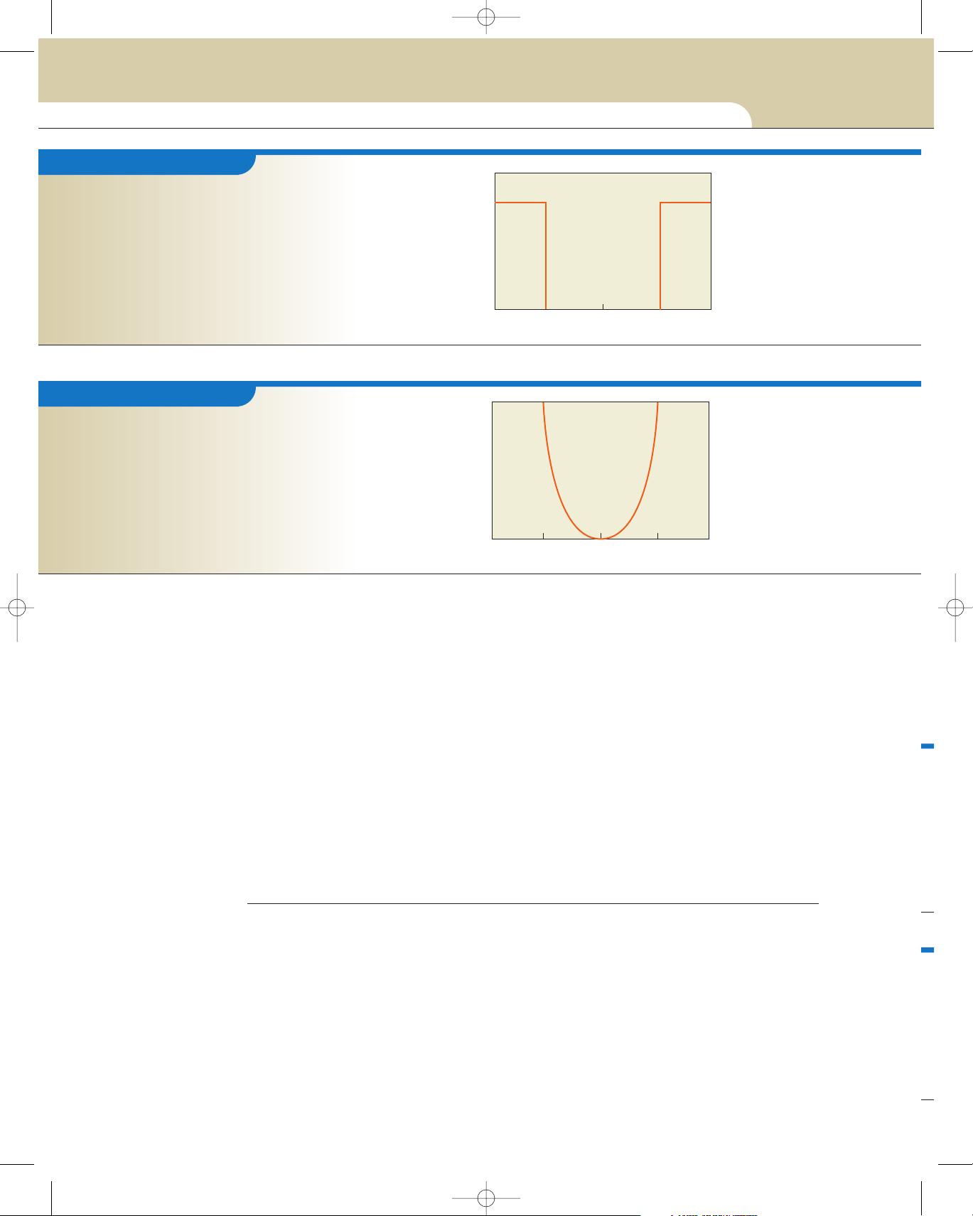
A traditional way of interpreting such a specification is that any part that falls within the
allowed range is equally good, whereas any part falling outside the range is totally bad.
This is illustrated in Exhibit TN7.1. (Note that the cost is zero over the entire specification
range, and then there is a quantum leap in cost once the limit is violated.)
Genichi Taguchi, a noted quality expert from Japan, has pointed out that the traditional
view illustrated in Exhibit TN7.1 is nonsense for two reasons:
1 From the customer’s view, there is often practically no difference between a product
just inside specifications and a product just outside. Conversely, there is a far greater
difference in the quality of a product that is the target and the quality of one that is
near a limit.
2 As customers get more demanding, there is pressure to reduce variability. However,
Exhibit TN7.1 does not reflect this logic.
Taguchi suggests that a more correct picture of the loss is shown in Exhibit TN7.2.
Notice that in this graph the cost is represented by a smooth curve. There are dozens of
Upper and lower specification
or tolerance limits
cha06369_tn07.qxd 2/12/03 7:01 PM Page 301
302 section 2 PRODUCT DESIGN AND PROCESS SELECTION
illustrations of this notion: the meshing of gears in a transmission, the speed of photo-
graphic film, the temperature in a workplace or department store. In nearly anything that
can be measured, the customer sees not a sharp line, but a gradation of acceptability away
from the “Aim” specification. Customers see the loss function as Exhibit TN7.2 rather than
Exhibit TN7.1.
Of course, if products are consistently scrapped when they are outside specifications,
the loss curve flattens out in most cases at a value equivalent to scrap cost in the ranges
outside specifications. This is because such products, theoretically at least, will never be
sold so there is no external cost to society. However, in many practical situations, either the
process is capable of producing a very high percentage of product within specifications
and 100 percent checking is not done, or if the process is not capable of producing within
specifications, 100 percent checking is done and out-of-spec products can be reworked to
bring them within specs. In any of these situations, the parabolic loss function is usually a
reasonable assumption.
PROCESS CAPABILITY
● ● ●
Taguchi argues that being within tolerance is not a yes/no decision, but rather a
continuous function. The Motorola quality experts, on the other hand, argue that the process
used to produce a good or deliver a service should be so good that the probability of gener-
ating a defect should be very, very low. Motorola made process capability and product
design famous by adopting six-sigma limits. When we design a part, we specify that certain
dimensions should be within the upper and lower tolerance limits.
As a simple example, assume that we are designing a bearing for a rotating shaft—say
an axle for the wheel of a car. There are many variables involved for both the bearing and
the axle—for example, the width of the bearing, the size of the rollers, the size of the axle,
the length of the axle, how it is supported, and so on. The designer specifies tolerances for
each of these variables to ensure that the parts will fit properly. Suppose that initially a
E XHIBIT TN7 . 1
A Traditional View of the Cost
of Variability
High
Zero
Incremental
cost to
society of
variability
Lower
spec
Upper
spec
Aim
spec
E XHIBIT TN7 . 2
Taguchi’s View of the Cost of
Variability
Incremental
cost to
society of
variability
Lower
spec
Upper
spec
Aim
spec
Zero
High
cha06369_tn07.qxd 2/12/03 7:01 PM Page 302
PROCESS CAPABILITY AND STATISTICAL QUALITY CONTROL technical note 303
design is selected and the diameter of the bearing is set at 1.250 inches
±0.005 inch. This means that acceptable parts may have a diameter that
varies between 1.245 and 1.255 inches (which are the lower and upper
tolerance limits).
Next, consider the process in which the bearing will be made. Let’s say
that by running some tests, we determine the machine output to have a
standard deviation or sigma equal to 0.002 inch. What this means is that
our process does not make each bearing exactly the same size. Assume that
we are monitoring the process such that any bearings that are more than
three standard deviations (
±0.006
inch) above or below 1.250 inches are
rejected. This means that we will produce parts that vary between 1.244
and 1.256 inches. As we can see, our process limits are greater than the tol-
erance limits specified by our designer. This is not good, because we will
produce some parts that do not meet specifications.
Motorola insists that a process making a part must be capable of operat-
ing so that the design tolerances are six standard deviations away from the
process mean. For our bearing, this would mean that our process variation
would need to be less than or equal to 0.00083 inch (remember our toler-
ance was ±0.005, which, when divided by 6, is 0.00083). To reduce the
variation in the process, we would need to find some better method for con-
trolling the formation of the bearing. Of course, another option would be to
redesign the axle assembly so that such perfect bearings are not needed.
We can show the six-sigma limits using an exhibit. Assume that we have
changed the process to produce with 0.00083 variation. Now, the design
limits and the process limits are acceptable according to Motorola stan-
dards. Let’s assume that the bearing diameter follows a bell-shaped normal distribution as
in Exhibit TN7.3. From our knowledge of the normal distribution, we know that 99.7 per-
cent of the bell-shaped curve falls within ±3 sigma. We would expect only about three
parts in 1,000 to fall outside of the three-sigma limits. The tolerance limits are another three
sigma out from these control limits! In this case, the actual number of parts we would
expect to produce outside the tolerance limits is only two parts per billion!
Suppose the central value of the process output shifts away from the mean. Exhibit TN7.4
shows the mean shifted one standard deviation closer to the upper specification limit. This
E XHIBIT TN7 . 3
Process Capability
Standard deviation ()
–6
Lower
tolerance
limit
–5 –4 –3 –2 –10123456
Upper
tolerance
limit
E XHIBIT TN7 . 4
Process Capability with a Shift
in the Process Mean
–6
Lower
tolerance
limit
–5 –4 –3 –2 –10123456
Upper
tolerance
limit
cha06369_tn07.qxd 2/12/03 7:01 PM Page 303
剩余22页未读,继续阅读
资源评论
tonybo2015
- 粉丝: 0
- 资源: 1
上传资源 快速赚钱
- 我的内容管理 展开
- 我的资源 快来上传第一个资源
- 我的收益 登录查看自己的收益
- 我的积分 登录查看自己的积分
- 我的C币 登录后查看C币余额
- 我的收藏
- 我的下载
- 下载帮助
安全验证
文档复制为VIP权益,开通VIP直接复制
信息提交成功