没有合适的资源?快使用搜索试试~ 我知道了~
最新《生成式对抗网络异常检测》综述论文
需积分: 0 11 下载量 169 浏览量
2021-09-16
17:28:52
上传
评论 2
收藏 1.17MB PDF 举报
温馨提示
试读
16页
异常检测是许多研究领域所面临的重要问题。探测并正确地将一些看不见的东西分类为异常是一个具有挑战性的问题,多年来已经通过许多不同的方式解决了这个问题。生成对抗网络(GANs)和对抗训练过程最近被用来面对这一任务,产生了显著的结果。在本文中,我们综述了主要的基于GAN的异常检测方法,并突出了它们的优缺点。在不同数据集上的实验结果的增加,以及使用GAN的异常检测的完整开源工具箱的公开发布。
资源推荐
资源详情
资源评论
A Survey on GANs for Anomaly Detection
Federico Di Mattia
1 *
Paolo Galeone
1 *
Michele De Simoni
1 *
Emanuele Ghelfi
1 *
Abstract
Anomaly detection is a significant problem faced
in several research areas. Detecting and correctly
classifying something unseen as anomalous is
a challenging problem that has been tackled in
many different manners over the years. Gener-
ative Adversarial Networks (GANs) and the ad-
versarial training process have been recently em-
ployed to face this task yielding remarkable re-
sults. In this paper we survey the principal GAN-
based anomaly detection methods, highlighting
their pros and cons. Our contributions are the
empirical validation of the main GAN models
for anomaly detection, the increase of the experi-
mental results on different datasets and the public
release of a complete Open Source toolbox for
Anomaly Detection using GANs.
1. Introduction
Anomalies are patterns in data that do not conform to a
well-defined notion of normal behavior (Chandola et al.,
2009). Generative Adversarial Networks (GANs) and the
adversarial training framework (Goodfellow et al., 2014)
have been successfully applied to model complex and high
dimensional distribution of real-world data. This GAN char-
acteristic suggests they can be used successfully for anomaly
detection, although their application has been only recently
explored. Anomaly detection using GANs is the task of
modeling the normal behavior using the adversarial training
process and detecting the anomalies measuring an anomaly
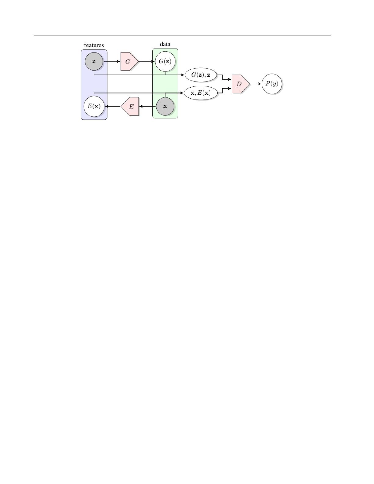
score (Schlegl et al., 2017). To the best of our knowledge,
all the GAN-based approaches to anomaly detection build
upon on the Adversarial Feature Learning idea (Donahue
et al., 2016) in which the BiGAN architecture has been
proposed. In their original formulation, the GAN frame-
work learns a generator that maps samples from an arbitrary
latent distribution (noise prior) to data as well as a discrimi-
nator which tries to distinguish between real and generated
samples. The BiGAN architecture extended the original for-
*
Equal contribution
1
Zuru Tech, Modena, Italy. Correspon-
dence to: Federico Di Mattia <federico.d@zuru.tech>.
mulation, adding the learning of the inverse mapping which
maps the data back to the latent representation. A learned
function that maps input data to its latent representation to-
gether with a function that does the opposite (the generator)
is the basis of the anomaly detection using GANs.
The paper is organized as follows. In Section 1 we introduce
the GANs framework and, briefly, its most innovative exten-
sions, namely conditional GANs and BiGAN, respectively
in Section 1.2 and Section 1.3. Section 2 contains the state
of the art architectures for anomaly detection with GANs.
In Section 3 we empirically evaluate all the analyzed archi-
tectures. Finally, Section 4 contains the conclusions and
future research directions.
1.1. GANs
GANs are a framework for the estimation of generative
models via an adversarial process in which two models, a
discriminator
D
and a generator
G
, are trained simultane-
ously. The generator
G
aim is to capture the data distribu-
tion, while the discriminator
D
estimates the probability that
a sample came from the training data rather than
G
. To learn
a generative distribution
p
g
over the data
x
the generator
builds a mapping from a prior noise distribution
p
z
to a data
space as
G(z; θ
G
)
, where
θ
G
are the generator parameters.
The discriminator outputs a single scalar representing the
probability that
x
came from real data rather than from
p
g
.
The generator function is denoted with
D(x; θ
D
)
, where
θ
D
are discriminator parameters.
The original GAN framework (Goodfellow et al., 2014)
poses this problem as a min-max game in which the two
players (
G
and
D
) compete against each other, playing the
following zero-sum min-max game:
min
G
max
D
V (D, G) = E
x∼p
data
(x)
[log D(x)]+
E
z∼p
z
(z)
[log (1 − D(G(z)))] .
(1)
1.2. Conditional GANs
GANs can be extended to a conditional model (Mirza &
Osindero, 2014) conditioning either
G
or
D
on some ex-
tra information
y
. The
y
condition could be any auxiliary
information, such as class labels or data from other modal-
ities. We can perform the conditioning by feeding
y
into
arXiv:1906.11632v2 [cs.LG] 14 Sep 2021
GANs for Anomaly Detection: a survey
Figure 1. The structure of BiGAN proposed in (Donahue et al., 2016).
both the discriminator and generator as an additional input
layer. The generator combines the noise prior
p
z
(z)
and
y
in a joint hidden representation, the adversarial training
framework allows for considerable flexibility in how this
hidden representation is composed. In the discriminator,
x
and
y
are presented as inputs to a discriminative function.
The objective function considering the condition becomes:
min
G
max
D
V (D, G) = E
x∼p
data
(x|y)
[log D(x)]+
E
z∼p
z
(z)
[log(1 − D(G(z|y)))].
(2)
1.3. BiGAN
Bidirectional GAN (Donahue et al., 2016) extends the GAN
framework including an encoder
E(x; θ
E
)
that learns the
inverse of the generator
E = G
−1
. The BiGAN training
process allows learning a mapping simultaneously from
latent space to data and vice versa. The encoder
E
is a
non-linear parametric function in the same way as
G
and
D
, and it can be trained using gradient descent. As in the
conditional GANs scenario, the discriminator must learn to
classify not only real and fake samples, but pairs in the form
(G(z), z) or (x, E(x)). The BiGAN training objective is:
min
G,E
max
D
V (D, G, E) =
E
x∼p
data
(x)
[E
z∼p
E(z|x)
[log D(x, z)]]+
E
z∼p
z
(z)
[E
x∼p
G
(x|z)
[log(1 − D(x, z)))]].
(3)
Figure 1 depicts a visual structure of the BiGAN architec-
ture.
2. GANs for anomaly detection
Anomaly detection using GANs is an emerging research
field. Schlegl et al. (2017), here referred to as AnoGAN,
were the first to propose such a concept. In order to face the
performance issues of AnoGAN a BiGAN-based approach
has been proposed in Zenati et al. (2018), here referred as
EGBAD (Efficient GAN Based Anomaly Detection), that
outperformed AnoGAN execution time. Recently, Akcay
et al. (2018) advanced a GAN + autoencoder based approach
that exceeded EGBAD performance from both evaluation
metrics and execution speed.
In the following sections, we present an analysis of the
considered architecture. The term sample and image are
used interchangeably since GANs can be used to detect
anomalies on a wide range of domains, but all the analyzed
architectures focused mostly on images.
2.1. AnoGAN
AnoGAN aim is to use a standard GAN, trained only on
positive samples, to learn a mapping from the latent space
representation
z
to the realistic sample
ˆ
x = G(z)
and use
this learned representation to map new, unseen, samples
back to the latent space. Training a GAN on normal samples
only, makes the generator learn the manifold
X
of normal
samples. Given that the generator learns how to generate
normal samples, when an anomalous image is encoded its
reconstruction will be non-anomalous; hence the difference
between the input and the reconstructed image will highlight
the anomalies. The two steps of training and detecting
anomalies are summarized in Figure 2.
The authors have defined the mapping of input samples to
the latent space as an iterative process. The aim is to find a
point
z
in the latent space that corresponds to a generated
value
G(z)
that is similar to the query value
x
located on
the manifold
X
of the positive samples. The research pro-
cess is defined as the minimization trough
γ = 1, 2, . . . , Γ
backpropagation steps of the loss function defined as the
weighted sum of the residual loss
L
R
and discriminator loss
L
D
, in the spirit of Yeh et al. (2016).
The residual loss measures the dissimilarity between the
query sample and the generated sample in the input domain
GANs for Anomaly Detection: a survey
Figure 2.
AnoGAN (Schlegl et al., 2017). The GAN is trained on positive samples. At test time, after
Γ
research iteration the latent vector
that maps the test image to its latent representation is found
z
Γ
. The reconstructed image
G(z
Γ
)
is used to localize the anomalous regions.
space:
L
R
(z
γ
) = ||x − G(z
γ
)||
1
. (4)
The discriminator loss takes into account the discriminator
response. It can be formalized in two different ways. Follow-
ing the original idea of Yeh et al. (2016), hence feeding the
generated image
G(z
γ
)
into the discriminator and calculat-
ing the sigmoid cross-entropy as in the adversarial training
phase: this takes into account the discriminator confidence
that the input sample is derived by the real data distribution.
Alternatively, using the idea introduced by Salimans et al.
(2016), and used by the AnoGAN (Schlegl et al., 2017)
authors, to compute the feature matching loss, extracting
features from a discriminator layer
f
in order to take into
account if the generated sample has similar features of the
input one, by computing:
L
D
(z
γ
) = ||f (x) − f (G(z
γ
))||
1
, (5)
hence the proposed loss function is:
L(z
γ
) = (1 − λ) · L
R
(z
γ
) + γ · L
D
(z
γ
). (6)
Its value at the
Γ
-th step coincides with the anomaly score
formulation:
A(x) = L(z
Γ
). (7)
A(x)
has no upper bound; to high values correspond an
high probability of x to be anomalous.
It should be noted that the minimization process is required
for every single input sample x.
2.1.1. PROS AND CONS
Pros
•
Showed that GANs can be used for anomaly detection.
•
Introduced a new mapping scheme from latent space
to input data space.
•
Used the same mapping scheme to define an anomaly
score.
Cons
•
Requires
Γ
optimization steps for every new input: bad
test-time performance.
•
The GAN objective has not been modified to take into
account the need for the inverse mapping learning.
•
The anomaly score is difficult to interpret, not being in
the probability range.
2.2. EGBAD
Efficient GAN-Based Anomaly Detection (EGBAD) (Zenati
et al., 2018) brings the BiGAN architecture to the anomaly
detection domain. In particular, EGBAD tries to solve the
AnoGAN disadvantages using Donahue et al. (2016) and Du-
moulin et al. (2017) works that allows learning an encoder
E
able to map input samples to their latent representation
during the adversarial training. The importance of learning
E
jointly with
G
is strongly emphasized, hence Zenati et al.
(2018) adopted a strategy similar to the one indicated in
Donahue et al. (2016) and Dumoulin et al. (2017) in order
to try to solve, during training, the optimization problem
min
G,E
max
D
V (D, E, G)
where
V (D, E, G)
is defined
as in Equation 3. The main contribution of the EGBAD is
to allow computing the anomaly score without
Γ
optimiza-
tion steps during the inference as it happens in AnoGAN
(Schlegl et al., 2017).
2.3. GANomaly
Akcay et al. (2018) introduce the GANomaly approach. In-
spired by AnoGAN (Schlegl et al., 2017), BiGAN (Donahue
et al., 2016) and EGBAD (Zenati et al., 2018) they train a
generator network on normal samples to learn their mani-
fold
X
while at the same time an autoencoder is trained to
learn how to encode the images in their latent representa-
tion efficiently. Their work is intended to improve the ideas
of Schlegl et al. (2017), Donahue et al. (2016) and Zenati
GANs for Anomaly Detection: a survey
Real / Fake
Input/Output
Conv
LeakyReLU
BatchNorm
ConvTranspose
ReLU Tanh Softmax
Figure 3. GANomaly architecture and loss functions from (Akcay et al., 2018).
et al. (2018). Their approach only needs a generator and a
discriminator as in a standard GAN architecture.
Generator network
The generator network consists of
three elements in series, an encoder
G
E
a decoder
G
D
(both assembling an autoencoder structure) and another en-
coder
E
. The architecture of the two encoders is the same.
G
E
takes in input an image
x
and outputs an encoded ver-
sion
z
of it. Hence,
z
is the input of
G
D
that outputs
ˆx
,
the reconstructed version of
x
. Finally,
ˆx
is given as an
input to the encoder
E
that produces
ˆz
. There are two main
contributions from this architecture. First, the operating
principle of the anomaly detection of this work lies in the
autoencoder structure. Given that we learn to encode nor-
mal (non-anomalous) data (producing
z
) and given that we
learn to generate normal data (
ˆx
) starting from the encoded
representation
z
, when the input data
x
is an anomaly its
reconstruction will be normal. Because the generator will al-
ways produce a non-anomalous image, the visual difference
between the input
x
and the produced
ˆx
will be high and in
particular will spatially highlight where the anomalies are
located. Second, the encoder
E
at the end of the generator
structure helps, during the training phase, to learn to encode
the images in order to have the best possible representation
of x that could lead to its reconstruction ˆx.
Discriminator network
The discriminator network
D
is
the other part of the whole architecture, and it is, with the
generator part, the other building block of the standard GAN
architecture. The discriminator, in the standard adversarial
training, is trained to discern between real and generated
data. When it is not able to discern among them, it means
that the generator produces realistic images. The generator
is continuously updated to fool the discriminator. Refer
to Figure 3 for a visual representation of the architecture
underpinning GANomaly.
The GANomaly architecture differs from AnoGAN (Schlegl
et al., 2017) and from EGBAD (Zenati et al., 2018). In
Figure 4 the three architectures are presented.
Beside these two networks, the other main contribution of
GANomaly is the introduction of the generator loss as the
sum of three different losses; the discriminator loss is the
classical discriminator GAN loss.
Generator loss
The objective function is formulated by
combining three loss functions, each of which optimizes a
different part of the whole architecture.
Adversarial Loss The adversarial loss it is chosen to be the
feature matching loss as introduced in Schlegl et al. (2017)
and pursued in Zenati et al. (2018):
L
adv
= E
x∼p
X
||f(x) − E
x∼p
X
f(G(x))||
2
,
(8)
where
f
is a layer of the discriminator
D
, used to extract
a feature representation of the input . Alternatively, binary
cross entropy loss can be used.
Contextual Loss Through the use of this loss the genera-
tor learns contextual information about the input data. As
shown in (Isola et al., 2016) the use of the
L
1
norm helps to
obtain better visual results:
L
con
= E
x∼p
X
||x − G(x)||
1
.
(9)
Encoder Loss This loss is used to let the generator network
learn how to best encode a normal (non-anomalous) image:
剩余15页未读,继续阅读
资源评论
syp_net
- 粉丝: 158
- 资源: 1196
上传资源 快速赚钱
- 我的内容管理 展开
- 我的资源 快来上传第一个资源
- 我的收益 登录查看自己的收益
- 我的积分 登录查看自己的积分
- 我的C币 登录后查看C币余额
- 我的收藏
- 我的下载
- 下载帮助
最新资源
- 2%EF%BC%9A%E9%99%95%E8%A5%BF%E
- yyspdz62_944.apk
- SAP公司间采购EDI配置-如何触发自动MIRO.docx
- python197基于图像识别的仪表实时监控系统.rar
- I2C驱动SHT30温湿度传感器和LCD12864使用例程(RSCG12864B)
- python193中学地理-中国的江河湖泊教学网(django).rar
- python191基于时间序列分析的大气污染预测软件(django).rar
- python190基于人脸识别智能化小区门禁管理系统.rar
- python189某医院体检挂号系统.rar
- python179的企业物流管理系统(django).rar
资源上传下载、课程学习等过程中有任何疑问或建议,欢迎提出宝贵意见哦~我们会及时处理!
点击此处反馈
安全验证
文档复制为VIP权益,开通VIP直接复制
信息提交成功