ht. J. Preps. Ves. & Piping 65 ( 1996) 303-309
0 199.5 Elsevier Scrence Limited
ELSEVIER
0308-0161(94)00141-3
Printed in Northern Ireland. All rights reserved
030%0161/96/$09.50
Failure assessment diagrams for use in R6
assessments for austenitic components
R. A. Ainsworth
Nuclear Electric plc, Berkeley Technology Centre, Berkeley, Gloucestershire GL13 9PB, UK
The third revision of the defect assessment procedure R6 extended the scope
of earlier versions, which addressed high strength ferritic steels, to a more
general class of material behaviour. In particular, it allowed assessments to be
made of defective austenitic components. This paper reviews the background
to the R6 procedures and the various options in revision 3 for deriving the
failure assessment curve. The most complex option, termed option 3, involves
the derivation of failure assessment curves from J values. This option is
examined using experimental data from austenitic specimens of various
geometries and crack sizes, and using finite-element data including analysis of
a surface defect in a plate. It is demonstrated that option 3 curves lie close to
approximate material-specific curves, termed option 2, which are derived from
uniaxial stress/strain data. Option 2 curves are derived for austenitic steels and
weld metals over a wide range of temperatures. It is shown, particularly for
parent austenitic steels, that the material-specific curves are sensibly independ-
ent of temperature and are close to the general purpose, option 1, failure
assessment curve presented in R6. Thus, it is concluded that it is appropriate
to use the simple option 1 curve
components.
1
INTRODUCTION
Early versions of the R6 procedure’,* were
concerned with the initiation of fracture at
defects in components made of ferritic steel. The
strain hardening capacity of austenitic materials
and their ability to accommodate significant
amounts of ductile tearing made these early
versions unsuitable for the assessment of
austenitic components. Revision 3 of R6,3
hereinafter referred to simply as R6, remedied
this situation by allowing for the explicit
treatment of strain hardening properties and
including assessments of stable tearing.
This paper is concerned with the treatment of
strain hardening properties as addressed by the
various options in R6 for deriving the failure
assessment curve. The background to the
procedures in R6 is first briefly reviewed and
then the particular relevance of the options is
examined by comparison with experimental data
and finite-element analyses of austenitic specim-
ens and components.
for defect assessments of - austenitic
2 BACKGROUND TO THE R6
PROCEDURES
To apply the R6 procedures, two parameters
must be calculated for the particular load,
P,
applied to the component containing a defect of
size, a. These parameters are denoted
K,
and
L,
and are defined by:
K =K,(P, 4
r
KlC
(1)
L, = PIP&, us”) (2)
where
K,
is the elastic stress intensity factor,
K1,
is the fracture toughness, a,, is the yield stress
and
PL
is the value of
P
corresponding to plastic
collapse of the component. Having evaluated
K,
and
L,,
failure by fracture at the defect is
avoided provided the assessment point
(L,, K,)
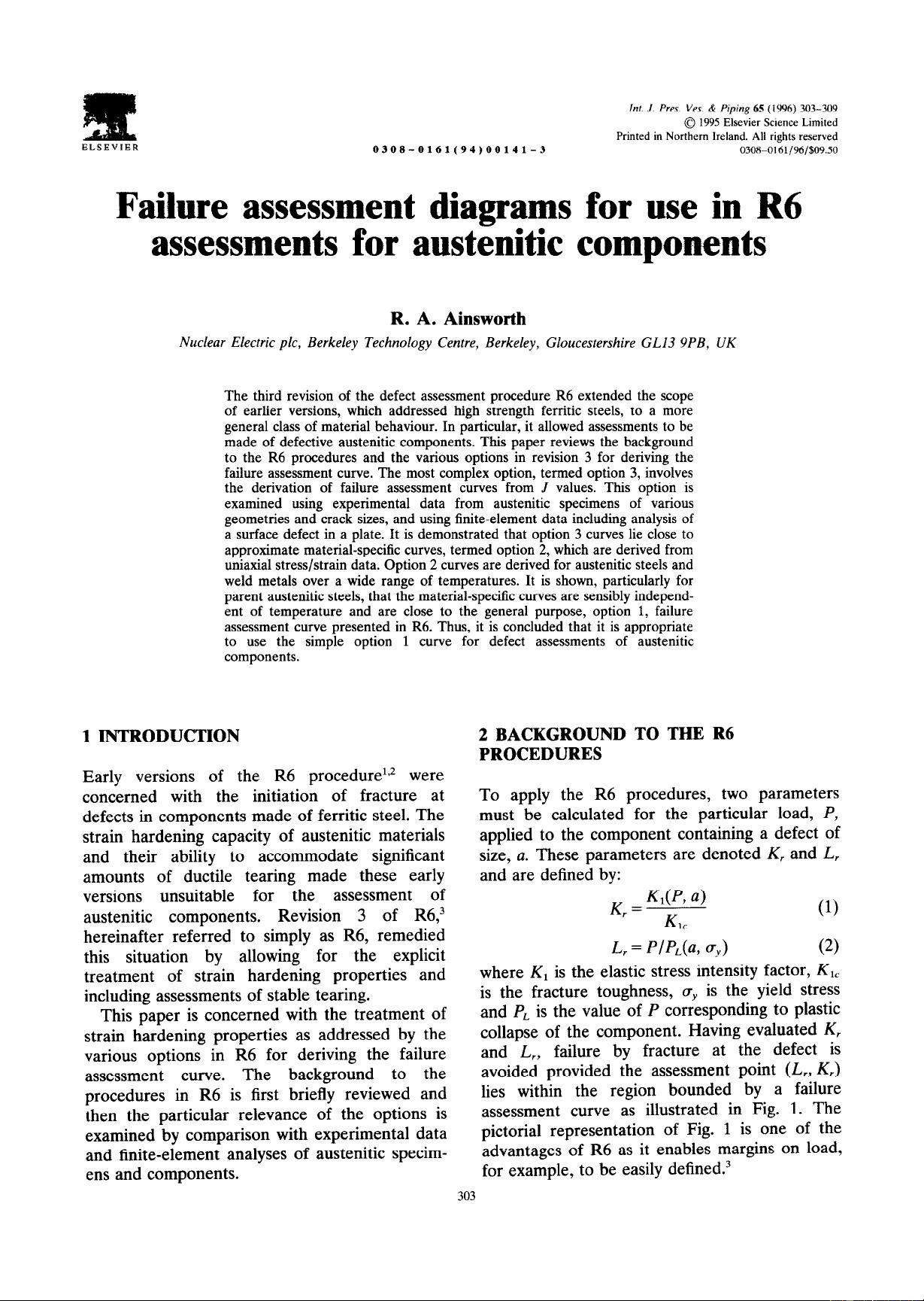
lies within the region bounded by a failure
assessment curve as illustrated in Fig. 1. The
pictorial representation of Fig. 1 is one of the
advantages of R6 as it enables margins on load,
for example, to be easily defined.3


 我的内容管理
展开
 我的资源
快来上传第一个资源
 我的收益 登录查看自己的收益
 我的积分
登录查看自己的积分
 我的C币
登录后查看C币余额
 我的收藏
我的收藏  我的下载
我的下载  下载帮助
下载帮助 
 前往需求广场,查看用户热搜

 信息提交成功