没有合适的资源?快使用搜索试试~ 我知道了~
资源推荐
资源详情
资源评论
Stupid Spherical Harmonics (SH)
Tricks
Peter-Pike Sloan
Microsoft Corporation
Abstract
This paper is a companion to a GDC 2008 Lecture with the same title. It provides a brief
overview of spherical harmonics (SH) and discusses several ways they can be used in interactive
graphics and problems that might arise. In particular it focuses on the following issues: How to
evaluate lighting models efficiently using SH, what “ringing” is and what you can do about it,
efficient evaluation of SH products and where they might be used. The most up to date version
is available on the web at
http://www.ppsloan.org/publications
Introduction
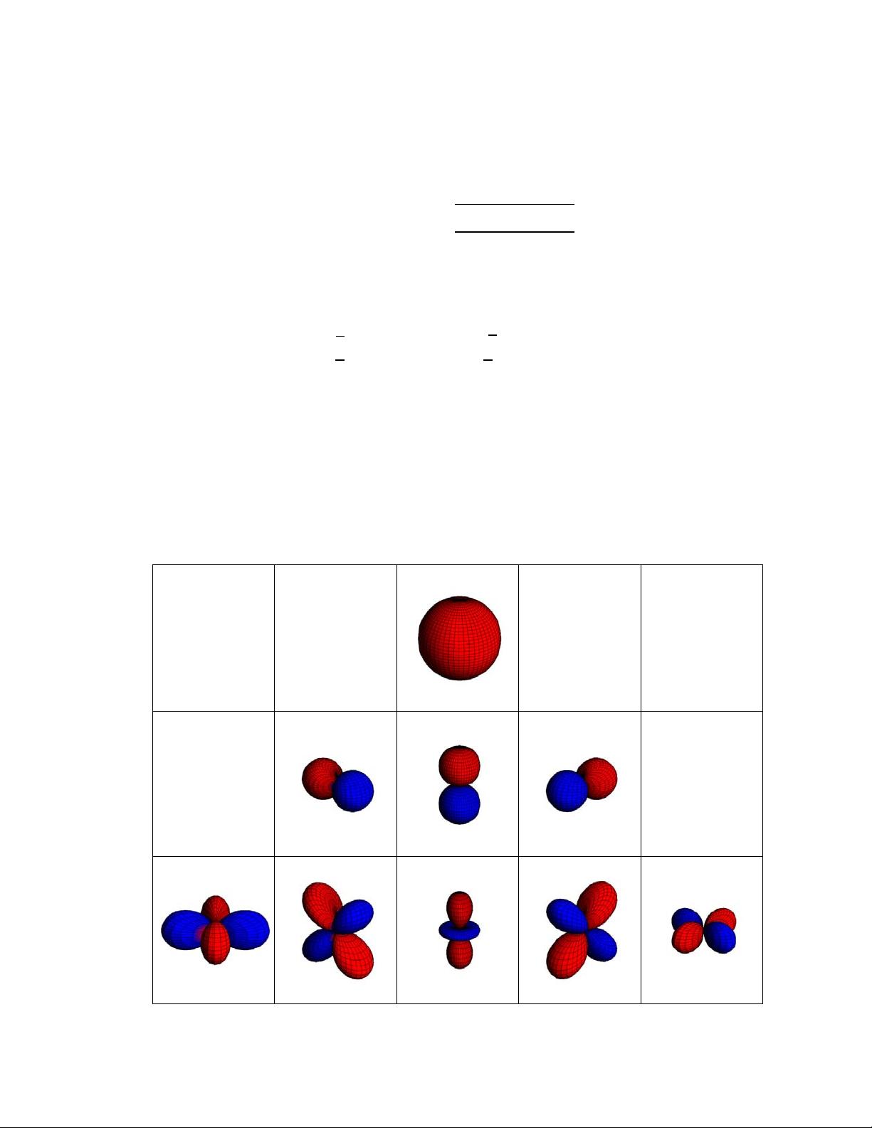
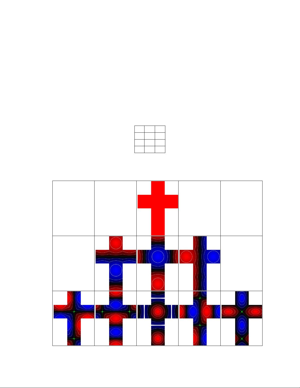
Harmonic functions [2], the solutions to Laplace’s equation, are used extensively in various
fields. Spherical Harmonics are the solutions when restricted to the sphere
1
[5]
. They have been
used to solve potential problems in physics, such as the heat equation (modeling the variation of
temperature over time [25]), and the gravitational and electric fields[9]. They have also been
used in quantum chemistry and physics to model the electron configuration in atoms and model
quantum angular momentum [16][51]. Closer to graphics they have been used to model
scattering phenomena [7][17]. In computer graphics they have been extensively used, early
uses were in modeling volumetric scattering effects [18], environmental reflections for micro-
facet BRDF’s without global shadows[6], non-diffuse off-line light transport simulations[40],
BRDF representations [53], image relighting[28], image based rendering with controllable
lighting [54][55], and modeling light source emission[8]. More recent examples include more
work in atmospheric scattering [50] and computer vision [3].
The focus of this article is on techniques related to interactive rendering. The first paper that
has been used extensively in games deals with using Spherical Harmonics to represent
irradiance environment maps efficiently, allowing for interactive rendering of diffuse objects
under distant illumination [35]. This was extended to handle a limited class of BRDF’s with the
same constraints [36]. Precomputed radiance transfer (PRT) [41][20][24] models a static
object/scenes response to a lighting environment, often represented using SH, including
complex global illumination effects like soft-shadows and inter-reflections with diffuse and
simple glossy materials. This was extended to handle more general BRDF models [20][23] [42],
1
They are the angular portion of the solution in spherical coordinates.
incorporate sub-surface scattering [42], significantly improve rendering efficiency through
compression techniques from machine learning [42], and various techniques to model “local”
texture like surface details [43][44][45]. SH have been used to model single scattering from
distant lighting environments [49]. Other uses have been in using gradients to lift the distant
lighting assumption [1], several techniques addressing dynamic objects [56][37] including
support for inter-reflections [46][33], as a representation of visibility to model shadowing of
objects with general BRDF models [12], using scaling operators to model shadows from
deformable objects [52], as a parameterization of refraction [11] and as a technique to address
the level of detail problem with normal maps [15].
More practical papers include covering implementation details for PRT [13], how to integrate
these techniques into an engine [30], how to use SH+gradients for irradiance volumes [31][32],
practical issues around projection and how to efficiently quantize SH coefficients [21] and a nice
paper that projects an analytic skylight model [34] into SH and uses a global polynomial fit to
evaluate the SH lightprobe as a function of the models parameters [14]. Numerical techniques
for more robustly projection functions defined over the hemisphere using SH have also been
investigated [22].
Many of the uses in real-time graphics are just as a convenient way for representing spherical
functions – visibility, lighting and reflectance. While there are many other basis functions that
can be used, wavelets [39], wavelets on cube maps [27], spherical radial basis functions [9], and
others [26], spherical harmonics have some nice properties that will be described in this
document. It is important to stress that there are scenarios where these other basis functions
are more appropriate.
While spherical harmonics may seem somewhat daunting, they are actually straightforward.
They are the spherical analog to the Fourier basis on the unit circle, and are easy to evaluate
numerically. Like the Fourier basis used in signal processing, care has to be taken when
truncating the series (which will always be done in video games), to minimize the “ringing”
artifacts that can occur. This article will describe how to evaluate and represent lights efficiently
using spherical harmonics, how to pull conventional lights out of a SH representation, describe
“ringing” and mitigation techniques to minimize its impact, and go over products of functions
using spherical harmonics, describing where they are useful and special cases that are worth
optimizing for.
Background
Definition Spherical Harmonics define an orthonormal
2
2
An orthonormal basis is one that has the property
=
, that is one if i==j, and zero otherwise.
basis over the sphere, S. Using the
parameterization
=
(
, ,
)
=
(
sin cos , sin sin , cos
)
Where s are simply locations on the unit sphere. The basis functions are defined as
(
,
)
=
|
|
(
cos
)
, ,
Where
are the associated Legendre polynomials and
are the normalization constants
=
(
2+ 1
)(
|
|)
!
4
(
+
|
|)
!
The above definition is for the complex form (most commonly used in the non-graphics
literature), a real valued basis is given by the transformation
=
2
Re
(
)
2
Im
(
)
0
> 0
< 0
= 0
=
2
cos
(
cos
)
2
sin
|
|
|
|
(
cos
)
0
0
(
cos
)
> 0
< 0
= 0
The index l represents the “band”. Each band is equivalent to polynomials of that degree (so
zero is just a constant function, 1 is linear, etc.) and there are 2l+1 functions in a given band.
While spherical coordinates are convenient when computing integrals, they can also be
represented using polynomials, as is commonly done when evaluating them (see Appendix A1
Recursive Rules for Evaluating SH Basis Functions and Appendix A2 Polynomial Forms of SH Basis
for details.) An order n SH expansion uses all of the basis functions through degree n-1.
Spherical Harmonics can be visualized in a couple of ways. One standard way is to distort a unit
sphere, by scaling each point radialy by the absolute value of the function and coloring it based
on the sign (red for positive, blue for negative.) Above are images of the first three bands using
this technique.
The functions in the central column (l=0) are called zonal harmonics (ZH) and will be discussed
later, these functions have rotational symmetry around the z axis and the zeros (locations where
the function is zero) are contours on the sphere parallel to the XY plane. The functions where
(l=|m|) are called sectorial harmonics and the zeros define regions like apple slices.
An alternative visualization is to draw them using the parameterization of a cube map unfolded
onto the plane. The unfolding of the cube map is as follows:
+Y
-X -Z +x
-Y
+Z
Here magnitude is encoded with color (red positive, blue negative, zero green) and iso-intensity
contours have been evenly placed (white lines) to give more intuition for the gradient of the
function (when they bunch together the function is changing faster, etc.)
Projection and Reconstruction Because the SH basis is orthonormal the least squares
projection of a scalar function f defined over S is done by simply integrating the function you
want to project,
(
)
, against the basis functions (proof in Appendix A6 Least Squares
Projection)
=
(
)
(
)
These coefficients can be used to reconstruct an approximation of the function f
(
)
=
(
)
=
=0
Which is increasingly accurate as the number of bands n increases. This paper concentrates on
low-frequency approximations to f, for higher frequency representations other bases tend to do
a better job. Projection to n-th order generates n
2
coefficients. It is often convenient to use a
single index for both the projection coefficients and the basis function, via
(
)
=
(
)
2
=0
Where i=l(l+1)+m . This formulation makes it clear that evaluating at direction s of the
approximate function is simply a dot product between the n
2
coefficient vector f
i
and the vector
of evaluated basis functions y
i
(s). The first coefficient (
0
0
or
0
depending on indexing)
represents the average value of the function over the sphere and will sometimes be referred to
as the DC term.
Basic Properties One important property of SH is how projections interact with rotations.
Given a function g(s), which represents a function f(s) rotated by a rotation matrix Q, so g(s) =
f(Q(s)) the projection of g is identical to rotating
and re-projecting it. This rotational
invariance is similar to the translational invariance in the Fourier transform. This means that, for
example, lighting will be stable under rotations, so there won’t be any aliasing artifacts or
“wobbling” of the light sources. Below are images of a sphere illuminated by a directional light
source, the top row is using SH, the bottom row is using the Ambient Cube basis
3
[26]
from Valve
. The first column is a best case orientation, and the second is near a worst case one. The
image is invariant using SH. This basis is discussed in more details in Appendix A9 Ambient Cube
Basis. This will happen to some extent with any other basis defined over the sphere.
3
This basis is more efficient to evaluate compared to SH, having 6 basis functions with only 3 being non-
zero at any point on the sphere.
剩余41页未读,继续阅读
资源评论
风流不在人知
- 粉丝: 8
- 资源: 14
上传资源 快速赚钱
- 我的内容管理 展开
- 我的资源 快来上传第一个资源
- 我的收益 登录查看自己的收益
- 我的积分 登录查看自己的积分
- 我的C币 登录后查看C币余额
- 我的收藏
- 我的下载
- 下载帮助
安全验证
文档复制为VIP权益,开通VIP直接复制
信息提交成功