没有合适的资源?快使用搜索试试~ 我知道了~
1706.05296v1.pdf
需积分: 0 0 下载量 111 浏览量
2024-04-30
10:28:04
上传
评论
收藏 8.15MB PDF 举报
温馨提示
试读
17页
1706.05296v1.pdf
资源推荐
资源详情
资源评论
Value-Decomposition Networks For Cooperative
Multi-Agent Learning
Peter Sunehag
DeepMind
Guy Lever
DeepMind
guylev[email protected]
Audrunas Gruslys
DeepMind
Wojciech Marian Czarnecki
DeepMind
Vinicius Zambaldi
DeepMind
Max Jaderberg
DeepMind
Marc Lanctot
DeepMind
Nicolas Sonnerat
DeepMind
Joel Z. Leibo
DeepMind
Karl Tuyls
DeepMind & University of Liverpool
Thore Graepel
DeepMind
Abstract
We study the problem of cooperative multi-agent reinforcement learning with a
single joint reward signal. This class of learning problems is difficult because of
the often large combined action and observation spaces. In the fully centralized
and decentralized approaches, we find the problem of spurious rewards and a
phenomenon we call the “lazy agent” problem, which arises due to partial observ-
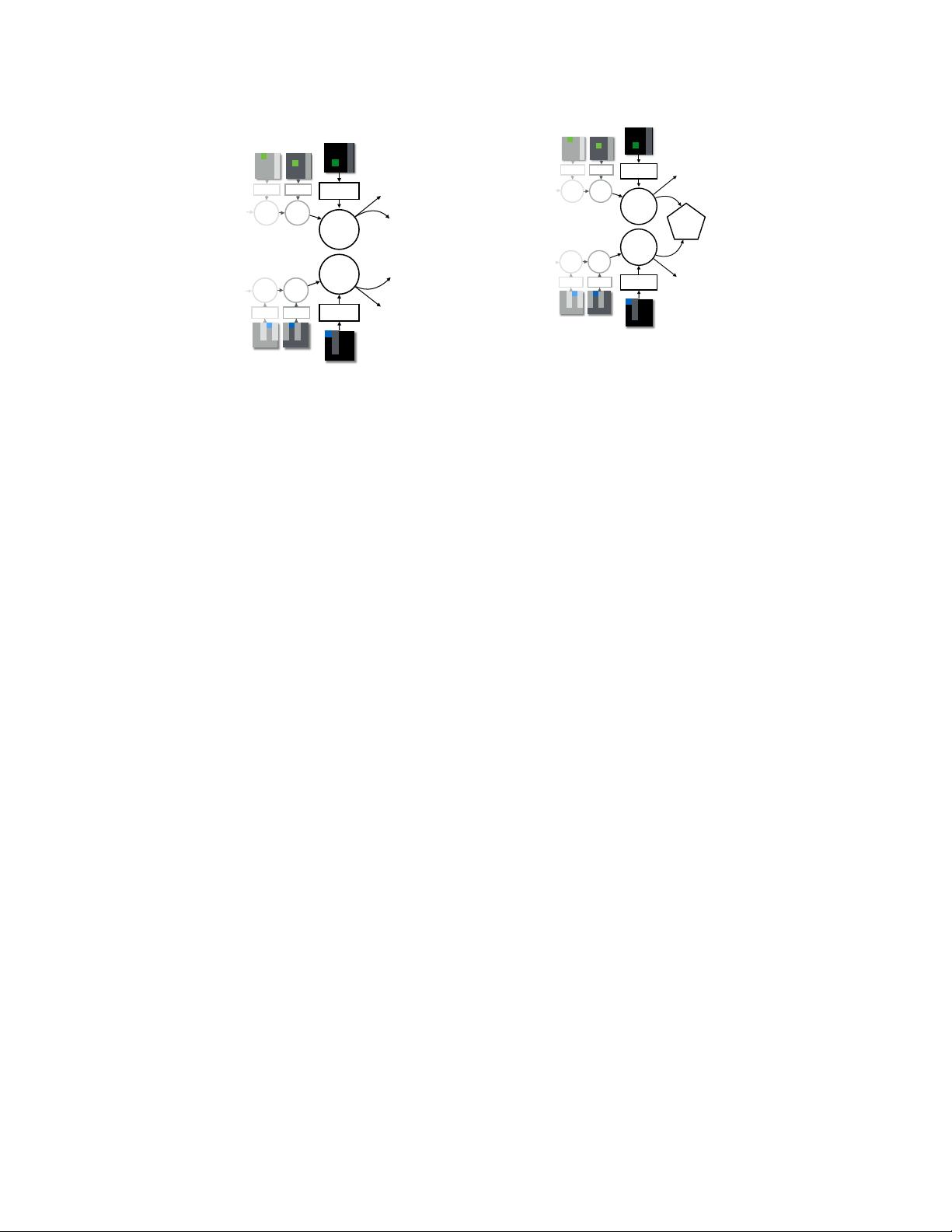
ability. We address these problems by training individual agents with a novel value
decomposition network architecture, which learns to decompose the team value
function into agent-wise value functions. We perform an experimental evaluation
across a range of partially-observable multi-agent domains and show that learning
such value-decompositions leads to superior results, in particular when combined
with weight sharing, role information and information channels.
1 Introduction
We consider the cooperative multi-agent reinforcement learning (MARL) problem (Panait and Luke,
2005; Busoniu et al., 2008; Tuyls and Weiss, 2012), in which a system of several learning agents must
jointly optimize a single reward signal – the team reward – accumulated over time. Each agent has
access to its own (“local”) observations and is responsible for choosing actions from its own action
set. Coordinated MARL problems emerge in applications such as coordinating self-driving vehicles
and/or traffic signals in a transportation system, or optimizing the productivity of a factory comprised
of many interacting components. More generally, with AI agents becoming more pervasive, they will
have to learn to coordinate to achieve common goals.
Although in practice some applications may require local autonomy, in principle the cooperative
MARL problem could be treated using a centralized approach, reducing the problem to single-agent
reinforcement learning (RL) over the concatenated observations and combinatorial action space.
We show that the centralized approach consistently fails on relatively simple cooperative MARL
arXiv:1706.05296v1 [cs.AI] 16 Jun 2017
problems in practice. We present a simple experiment in which the centralised approach fails by
learning inefficient policies with only one agent active and the other being “lazy”. This happens
when one agent learns a useful policy, but a second agent is discouraged from learning because its
exploration would hinder the first agent and lead to worse team reward.
1
An alternative approach is to train independent learners to optimize for the team reward. In general
each agent is then faced with a non-stationary learning problem because the dynamics of its envi-
ronment effectively changes as teammates change their behaviours through learning (Laurent et al.,
2011). Furthermore, since from a single agent’s perspective the environment is only partially ob-
served, agents may receive spurious reward signals that originate from their teammates’ (unobserved)
behaviour. Because of this inability to explain its own observed rewards naive independent RL is
often unsuccessful: for example Claus and Boutilier (1998) show that independent
Q
-learners cannot
distinguish teammates’ exploration from stochasticity in the environment, and fail to solve even an
apparently trivial, 2-agent, stateless,
3 × 3
-action problem and the general Dec-POMDP problem
is known to be intractable (Bernstein et al., 2000; Oliehoek and Amato, 2016). Though we here
focus on 2 player coordination, we note that the problems with individual learners and centralized
approaches just gets worse with more agents since then, most rewards do not relate to the individual
agent and the action space grows exponentially for the fully centralized approach.
One approach to improving the performance of independent learners is to design individual reward
functions, more directly related to individual agent observations. However, even in the single-agent
case, reward shaping is difficult and only a small class of shaped reward functions are guaranteed to
preserve optimality w.r.t. the true objective (Ng et al., 1999; Devlin et al., 2014; Eck et al., 2016). In
this paper we aim for more general autonomous solutions, in which the decomposition of the team
value function is learned.
We introduce a novel
learned additive value-decomposition
approach over individual agents. Im-
plicitly, the value decomposition network aims to learn an optimal linear value decomposition from
the team reward signal, by back-propagating the total
Q
gradient through deep neural networks repre-
senting the individual component value functions. This additive value decomposition is specifically
motivated by avoiding the spurious reward signals that emerge in purely independent learners.The
implicit value function learned by each agent depends only on local observations, and so is more
easily learned. Our solution also ameliorates the coordination problem of independent learning
highlighted in Claus and Boutilier (1998) because it effectively learns in a centralised fashion at
training time, while agents can be deployed individually.
Further, in the context of the introduced agent, we evaluate weight sharing, role information and
information channels as additional enhancements that have recently been reported to improve sample
complexity and memory requirements (Hausknecht, 2016; Foerster et al., 2016; Sukhbaatar et al.,
2016). However, our main comparison is between three kinds of architecture; Value-Decomposition
across individual agents, Independent Learners and Centralized approaches. We investigate and
benchmark combinations of these techniques applied to a range of new interesting two-player
coordination domains. We find that Value-Decomposition is a much better performing approach than
centralization or fully independent learners, and that when combined with the additional techniques,
results in an agent that consistently outperforms centralized and independent learners by a big margin.
1.1 Other Related Work
Schneider et al. (1999) consider the optimization of the sum of individual reward functions, by
optimizing local compositions of individual value functions learnt from them. Russell and Zimdars
(2003) sums the
Q
-functions of independent learning agents with individual rewards, before making
the global action selection greedily to optimize for total reward. Our approach works with only a
team reward, and learns the value-decomposition autonomously from experience, and it similarly
differs from the approach with coordination graphs (Guestrin et al., 2002) and the max-plus algorithm
(Kuyer et al., 2008; van der Pol and Oliehoek, 2016).
Other work addressing team rewards in cooperative settings is based on difference rewards (Tumer
and Wolpert, 2004), measuring the impact of an agent’s action on the full system reward. This reward
1
For example, imagine training a 2-player soccer team using RL with the number of goals serving as the team
reward signal. Suppose one player has become a better scorer than the other. When the worse player takes a shot
the outcome is on average much worse, and the weaker player learns to avoid taking shots (Hausknecht, 2016).
2
has nice properties (e.g. high learnability), but can be impractical as it requires knowledge about
the system state (Colby et al., 2016; Agogino and Tumer, 2008; Proper and Tumer, 2012). Other
approaches can be found in Devlin et al. (2014); HolmesParker et al. (2016); Babes et al. (2008).
2 Background
2.1 Reinforcement Learning
We recall some key concepts of the RL setting (Sutton and Barto, 1998), an agent-environment
framework (Russell and Norvig, 2010) in which an agent sequentially interacts with the environment
over a sequence of timesteps,
t = 1, 2, 3, . . .
, by executing actions and receiving observations
and rewards, and aims to maximize cumulative reward. This is typically modelled as a Markov
decision process (MDP) (e.g. Puterman, 1994) defined by a tuple
hS, A, T
1
, T , Ri
comprising the
state space
S
, action space
A
, a (possibly stochastic) reward function
R : S × A × S → R
start
state distribution
T
1
∈ P(S)
and transition function
T : S × A → P(S)
, where
P(X )
denotes the
set of probability distributions over the set
X
. We use
¯
R
to denote the expected value of
R
. The
agent’s interactions give rise to a trajectory
(S
1
, A
1
, R
1
, S
2
, ...)
where
S
1
∼ T
1
,
S
t+1
∼ T (·|S
t
, A
t
)
and
R
t
= R(S
t
, A
t
, S
t+1
)
, and we denote random variables in upper-case, and their realizations in
lower-case. At time
t
the agent observes
o
t
∈ O
which is typically some function of the state
s
t
, and
when the state is not fully observed the system is called a partially observed Markov decision process
(POMDP).
The agent’s goal is to maximize expected cumulative discounted reward with a discount factor
γ
,
R
t
:=
P
∞
t=1
γ
t−1
R
t
. The agent chooses actions according to a policy: a (stationary) policy
is a function
π : S → P(A)
from states to probability distributions over
A
. An optimal policy
is one which maximizes expected cumulative reward. In fully observed environments, stationary
optimal policies exist. In partially observed environments, the policy usually incorporates past agent
observations from the history
h
t
= a
1
o
1
r
1
, ..., a
t−1
o
t−1
r
t−1
(replacing
s
t
). A practical approach
utilized here, is to parameterize policies using recurrent neural networks.
V
π
(s) := E[
P
∞
t=1
γ
t−1
R(S
t
, A
t
, S
t+1
)|S
1
= s; A
t
∼ π(·|S
t
)]
is the value function and the action-
value function is
Q
π
(s, a) := E
S
0
∼T (·|s,a)
[R(S, a, S
0
)+γV (S
0
)]
(generally, we denote the successor
state of
s
by
s
0
). The optimal value function is defined by
V
∗
(s) = sup
π
V
π
(s)
and similarly
Q
∗
(s, a) = sup
π
Q
π
(s, a)
. For a given action-value function
Q : S × A → R
we define the
(deterministic) greedy policy w.r.t.
Q
by
π(s) := arg max
a∈A
Q(s, a)
(ties broken arbitrarily). The
greedy policy w.r.t. Q
∗
is optimal (e.g. Szepesvári, 2010).
2.2 Deep Q-Learning
One method for obtaining
Q
∗
is
Q
-learning which is based on the update
Q
i+1
(s
t
, a
t
) = (1 −
η
t
)Q
i
(s
t
, a
t
) + η
t
(r
t
+ γ max
a
Q
i
(s
t+1
, a))
, where
η
t
∈ (0, 1)
is the learning rate. We employ
the
ε
-greedy approach to action selection based on a value function, which means that with
1 − ε
probability we pick
arg max
a
Q
i
(s, a)
and with probability
ε
a random action. Our study focuses on
deep architectures for the value function similar to those used by Mnih et al. (2015), and our approach
incorporates the key techniques of target networks and experience replay employed there, making
the update into a stochastic gradient step. Since we consider partially observed environments our
Q
-functions are defined over agent observation histories,
Q(h
t
, a
t
)
, and we incorporate a recurrent
network similarly to Hausknecht and Stone (2015). To speed up learning we add the dueling
architecture of Wang et al. (2016) that represent
Q
using a value and an advantage function, including
multi-step updates with a forward view eligibility trace (e.g. Harb and Precup, 2016) over a certain
number of steps. When training agents the recurrent network is updated with truncated back-
propagation through time (BPTT) for this amount of steps. Although we concentrate on DQN-based
agent architectures, our techniques are also applicable to policy gradient methods such as A3C (Mnih
et al., 2016).
2.3 Multi-Agent Reinforcement Learning
We consider problems where observations and actions are distributed across
d
agents, and are
represented as d-dimensional tuples of primitive observations in O and actions in A. As is standard
3
a
1
a
2
Q
1
Q
2
o
2
t
o
1
t
o
2
t-1
o
2
t-2
o
1
t-1
o
1
t-2
Figure 1: Independent agents architecture showing
how local observations enter the networks of two
agents over time (three steps shown), pass through
the low-level linear layer to the recurrent layer, and
then a dueling layer produces individual
Q
-values.
a
1
a
2
Q
Q
1
Q
2
o
2
t
o
1
t
o
2
t-1
o
2
t-2
o
1
t-1
o
1
t-2
~
~
Figure 2: Value-decomposition individual architec-
ture showing how local observations enter the net-
works of two agents over time (three steps shown),
pass through the low-level linear layer to the re-
current layer, and then a dueling layer produces
individual "values" that are summed to a joint
Q
-
function for training, while actions are produced
independently from the individual outputs.
in MARL, the underlying environment is modeled as a Markov game where actions are chosen and
executed simultaneously, and new observations are perceived simultaneously as a result of a transition
to a new state (Littman, 1994, 2001; Hu and Wellman, 2003; Busoniu et al., 2008).
Although agents have individual observations and are responsible for individual actions, each agent
only receives the joint reward, and we seek to optimize
R
t
as defined above. This is consistent with
the Dec-POMDP framework (Oliehoek et al., 2008; Oliehoek and Amato, 2016).
If we denote
¯
h := (h
1
, h
2
, ..., h
d
)
a tuple of agent histories, a joint policy is in general a map
π : H
d
→ P(A
d
)
; we in particular consider policies where for any history
¯
h
, the distribution
π(
¯
h)
has independent components in
P(A)
. Hence, we write
π : H
d
→ P(A)
d
. The exception is when
we use the most naive centralized agent with a combinatorial action space, aka joint action learners.
3 A Deep-RL Architecture for Coop-MARL
Building on purely independent DQN-style agents (see Figure 1), we add enhancements to overcome
the identified issues with the MARL problem. Our main contribution of value-decomposition is
illustrated by the network in Figure 2.
The main assumption we make and exploit is that the joint action-value function for the system can
be additively decomposed into value functions across agents,
Q((h
1
, h
2
, ..., h
d
), (a
1
, a
2
, ..., a
d
)) ≈
d
X
i=1
˜
Q
i
(h
i
, a
i
)
where the
˜
Q
i
depends only on each agent’s local observations. We learn
˜
Q
i
by backpropagating
gradients from the
Q
-learning rule using the joint reward through the summation, i.e.
˜
Q
i
is learned
implicitly rather than from any reward specific to agent
i
, and we do not impose constraints that
the
˜
Q
i
are action-value functions for any specific reward. The value decomposition layer can be
seen in the top-layer of Figure 2. One property of this approach is that, although learning requires
some centralization, the learned agents can be deployed independently, since each agent acting
greedily with respect to its local value
˜
Q
i
is equivalent to a central arbiter choosing joint actions by
maximizing the sum
P
d
i=1
˜
Q
i
.
4
剩余16页未读,继续阅读
资源评论
1496许褚
- 粉丝: 2
- 资源: 1
上传资源 快速赚钱
- 我的内容管理 展开
- 我的资源 快来上传第一个资源
- 我的收益 登录查看自己的收益
- 我的积分 登录查看自己的积分
- 我的C币 登录后查看C币余额
- 我的收藏
- 我的下载
- 下载帮助
安全验证
文档复制为VIP权益,开通VIP直接复制
信息提交成功