Sampling methods for uncertainty analysis
Simple random sampling
Simple random sampling involves repeatedly forming random vectors of parameters from
prescribed probability distributions. A normally-distributed random variable x with mean
µ
and standard deviation
σ
can be generated by:
x* =
σ
r
n
+
µ
where r
n
are normally distributed random numbers with mean 0 and variance 1.
A multivariate normal distribution with variance-covariance matrix V can be
sampled utilising the lower and upper triangular matrix (LU) decomposition method
(Davis, 1987). The variance-covariance matrix V is first decomposed by Cholesky
factorization:
V = L L
T
where L is the lower triangular matrix. To generate the random variables vector x,
matrix L is multiplied by vector, r
n
, of independent normal random numbers with mean 0
and variance 1:
x = L r
n
+ µ .
The procedure is repeated for sample size ns, resulting in a set of variables with
expected mean vector µ and expected variance-covariance matrix: L cov(r
n
) L
T
. Since
the random numbers are independent, the covariance matrix cov(r
n
) should equal I (the
identity matrix),
L cov(r
n
) L
T
= L I L
T
= L L
T
= V .
Latin hypercube sampling
Latin hypercube sampling (LHS), a stratified-random procedure, provides an efficient
way of sampling variables from their distributions (Iman and Conover, 1980). The LHS
involves sampling ns values from the prescribed distribution of each of k variables
X
1
, X
2
,
…
X
k
. The cumulative distribution for each variable is divided into N equiprobable
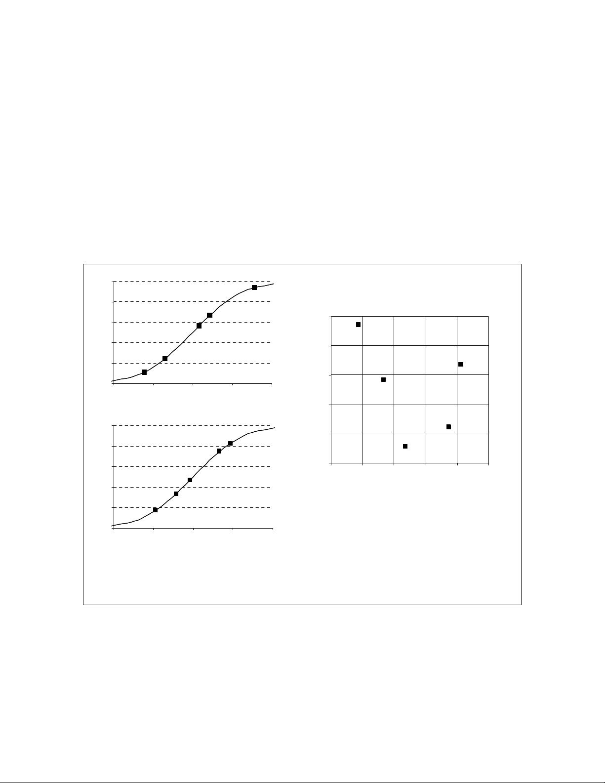
intervals. A value is selected randomly from each interval (Figure 1). The N values
obtained for each
variable are paired randomly with the other variables. Unlike simple
random sampling, this method ensures a full coverage of the range of each variable by
maximally stratifying each marginal distribution.
The LHS can be summarized as:
• divide the cumulative distribution of each variable into N equiprobable invervals;
• from each interval select a value randomly, for the ith interval, the sampled
cumulative probability can be written as (Wyss and Jorgensen, 1998):
Prob
i
= (1/N) r
u
+ (i – 1)/N
where r
u
is uniformly distributed random number ranging from 0 to 1;


