export_fig
==========
A toolbox for exporting figures from MATLAB to standard image and document formats nicely.
### Overview
Exporting a figure from MATLAB the way you want it (hopefully the way it looks on screen), can be a real headache for the unitiated, thanks to all the settings that are required, and also due to some eccentricities (a.k.a. features and bugs) of functions such as `print`. The first goal of export_fig is to make transferring a plot from screen to document, just the way you expect (again, assuming that's as it appears on screen), a doddle.
The second goal is to make the output media suitable for publication, allowing you to publish your results in the full glory that you originally intended. This includes embedding fonts, setting image compression levels (including lossless), anti-aliasing, cropping, setting the colourspace, alpha-blending and getting the right resolution.
Perhaps the best way to demonstrate what export_fig can do is with some examples.
### Examples
**Visual accuracy** - MATLAB's exporting functions, namely `saveas` and `print`, change many visual properties of a figure, such as size, axes limits and ticks, and background colour, in unexpected and unintended ways. Export_fig aims to faithfully reproduce the figure as it appears on screen. For example:
```Matlab
plot(cos(linspace(0, 7, 1000)));
set(gcf, 'Position', [100 100 150 150]);
saveas(gcf, 'test.png');
export_fig test2.png
```
generates the following:
| Figure: | test.png: | test2.png: |
|:-------:|:---------:|:----------:|
|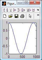|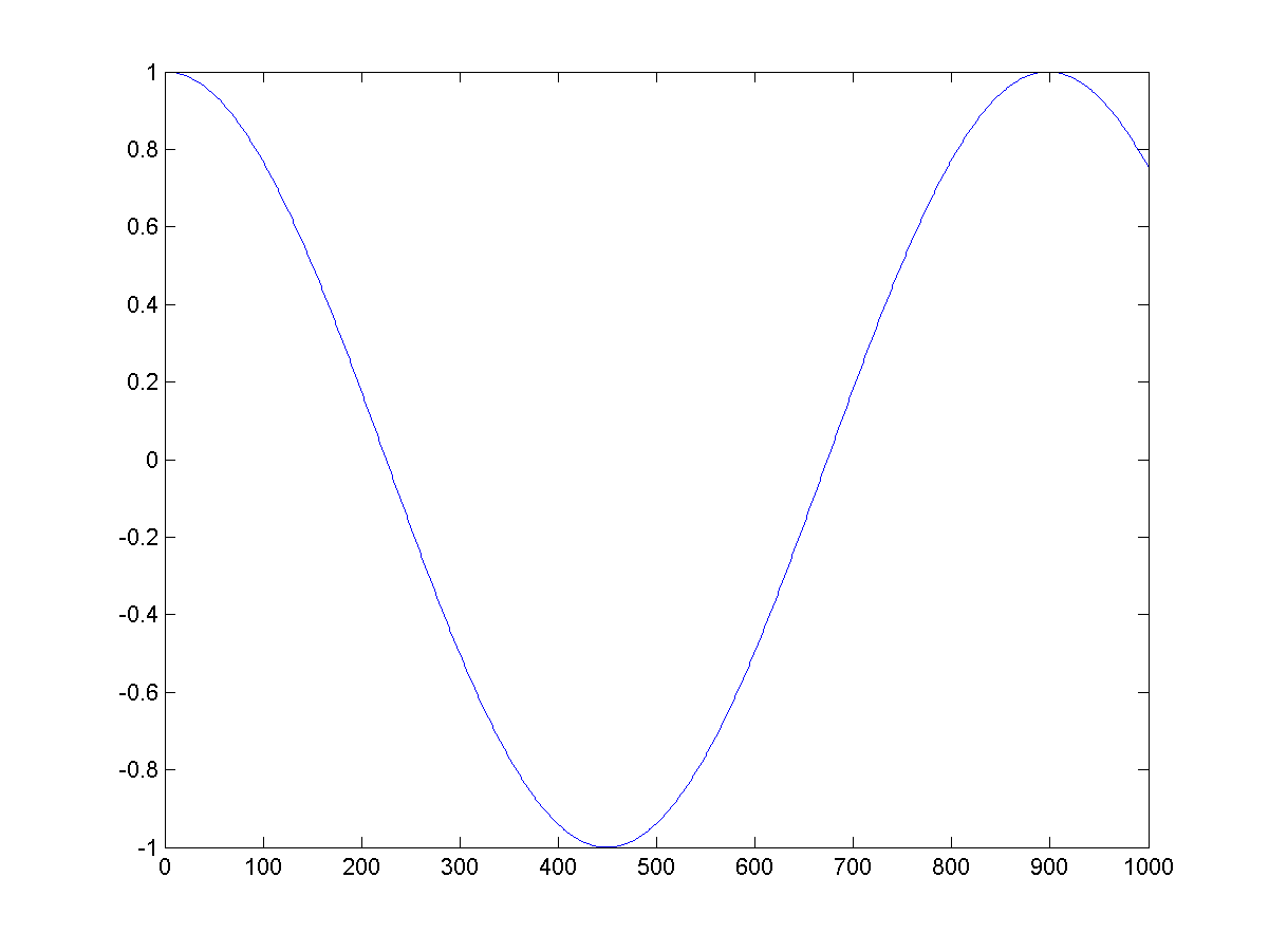||
Note that the size and background colour of test2.png (the output of export_fig) are the same as those of the on screen figure, in contrast to test.png. Of course, if you want the figure background to be white (or any other colour) in the exported file then you can set this prior to exporting using:
```Matlab
set(gcf, 'Color', 'w');
```
Notice also that export_fig crops and anti-aliases (smooths, for bitmaps only) the output by default. However, these options can be disabled; see the Tips section below for details.
**Resolution** - by default, export_fig exports bitmaps at screen resolution. However, you may wish to save them at a different resolution. You can do this using either of two options: `-m<val>`, where <val> is a positive real number, magnifies the figure by the factor <val> for export, e.g. `-m2` produces an image double the size (in pixels) of the on screen figure; `-r<val>`, again where <val> is a positive real number, specifies the output bitmap to have <val> pixels per inch, the dimensions of the figure (in inches) being those of the on screen figure. For example, using:
```Matlab
export_fig test.png -m2.5
```
on the figure from the example above generates:
Sometimes you might have a figure with an image in. For example:
```Matlab
imshow(imread('cameraman.tif'))
hold on
plot(0:255, sin(linspace(0, 10, 256))*127+128);
set(gcf, 'Position', [100 100 150 150]);
```
generates this figure:
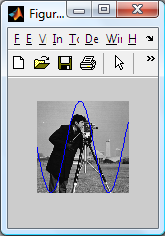
Here the image is displayed in the figure at resolution lower than its native resolution. However, you might want to export the figure at a resolution such that the image is output at its native (i.e. original) size (in pixels). Ordinarily this would require some non-trivial computation to work out what that resolution should be, but export_fig has an option to do this for you. Using:
```Matlab
export_fig test.png -native
```
produces:
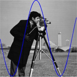
with the image being the size (in pixels) of the original image. Note that if you want an image to be a particular size, in pixels, in the output (other than its original size) then you can resize it to this size and use the `-native` option to achieve this.
All resolution options (`-m<val>`, `-q<val>` and `-native`) correctly set the resolution information in PNG and TIFF files, as if the image were the dimensions of the on screen figure.
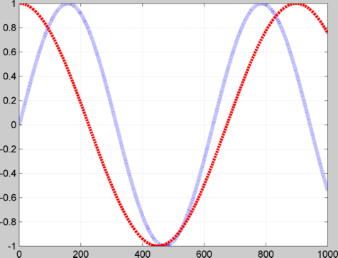
**Shrinking dots & dashes** - when exporting figures with dashed or dotted lines using either the ZBuffer or OpenGL (default for bitmaps) renderers, the dots and dashes can appear much shorter, even non-existent, in the output file, especially if the lines are thick and/or the resolution is high. For example:
```Matlab
plot(sin(linspace(0, 10, 1000)), 'b:', 'LineWidth', 4);
hold on
plot(cos(linspace(0, 7, 1000)), 'r--', 'LineWidth', 3);
grid on
export_fig test.png
```
generates:
This problem can be overcome by using the painters renderer. For example:
```Matlab
export_fig test.png -painters
```
used on the same figure generates:
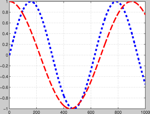
Note that not only are the plot lines correct, but the grid lines are too.
**Transparency** - sometimes you might want a figure and axes' backgrounds to be transparent, so that you can see through them to a document (for example a presentation slide, with coloured or textured background) that the exported figure is placed in. To achieve this, first (optionally) set the axes' colour to 'none' prior to exporting, using:
```Matlab
set(gca, 'Color', 'none'); % Sets axes background
```
then use export_fig's `-transparent` option when exporting:
```Matlab
export_fig test.png -transparent
```
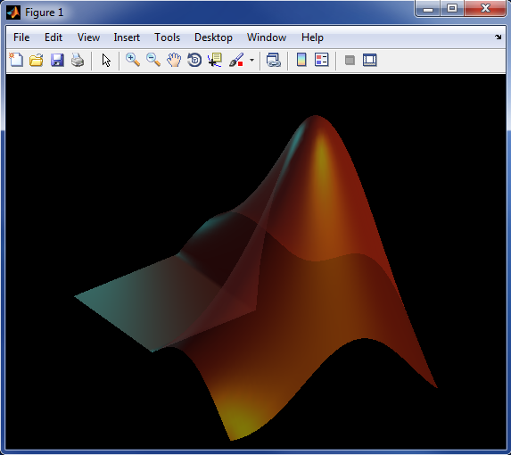
This will make the background transparent in PDF, EPS and PNG outputs. You can additionally save fully alpha-blended semi-transparent patch objects to the PNG format. For example:
```Matlab
logo;
alpha(0.5);
```
generates a figure like this:
If you then export this to PNG using the `-transparent` option you can then put the resulting image into, for example, a presentation slide with fancy, textured background, like so:
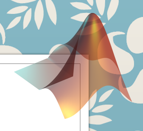
and the image blends seamlessly with the background.
**Image quality** - when publishing images of your results, you want them to look as good as possible. By default, when outputting to lossy file formats (PDF, EPS and JPEG), export_fig uses a high quality setting, i.e. low compression, for images, so little information is lost. This is in contrast to MATLAB's print and saveas functions, whose default quality settings are poor. For example:
```Matlab
A = im2double(imread('peppers.png'));
B = randn(ceil(size(A, 1)/6), ceil(size(A, 2)/6), 3) * 0.1;
B = cat(3, kron(B(:,:,1), ones(6)), kron(B(:,:,2), ones(6)), kron(B(:,:,3), ones(6)));
B = A + B(1:size(A, 1),1:size(A, 2),:);
imshow(B);
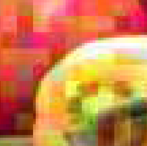
print -dpdf test.pdf
```
generates a PDF file, a sub-window of which looks (when zoomed in) like this:
while the command
```Matlab
export_fig test.pdf
```
on the same figure produces this:
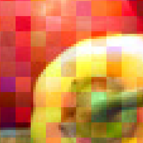
While much better, the image still contains some compression artifacts (see the low level noise around the edge of the pepper). You may prefer to export with no artifacts at all, i.e. lossless compression. Alternatively, you might need a smaller file, and be willing to accept more compression. Either way, export_fig has an option that can suit your needs: `-q<val>`, where <val> is a number from 0-100, will set the level of lossy image compression (again in PDF, EPS and JPEG outputs only; other formats are lossless), from high compression (0) to low compression/high quality (100). If you want lossless compression in any of those formats then specify a <val> greater than 100. For examp
模拟适用于欠驱动轻型张拉整体机器人辅助脊柱.zip

版权申诉
152 浏览量
2023-04-08
18:06:34
上传
评论
收藏 90.09MB ZIP 举报
 模拟适用于欠驱动轻型张拉整体机器人辅助脊柱.zip (772个子文件)
  mpc_org_e-4x1.4_40_from_-pi 0B affine-40-2e-4-eps-1e-5-0-pi 0B affine_200_2e-5_eps_1e-6_0-pi-8mat 143KB affine_80_1e-4_eps_1e-4_0-pi 0B affine_80_1e-5_eps_1e-4_0-pi 0B affine_revise_30_1e-4_eps_1e-5_0-pi 0B InvKin.asv 6KB ImageSelection.class 1KB spine_traj_end.eps 2.06MB spine_traj_start.eps 2.01MB plot_2d_spine_4cables.eps 1.02MB main_result_2-3-18.eps 229KB allvert_Feb2017.eps 180KB 2D_tracking_states_2017-04-16.eps 151KB all_errors_withdisturb_Feb2017.eps 133KB all_errors_nodisturb_Feb2017.eps 133KB forceplatemodel_Fy_topright.eps 133KB forceplatemodel_Fy_final.eps 132KB forceplatemodel_Fz_topright.eps 132KB forceplatemodel_Fz_toprightsym.eps 132KB forceplatemodel_Fz_topleftsym.eps 132KB forceplatemodel_test_09092016_202023.eps 114KB total_error_combined_Feb2017.eps 92KB zero_traj_LQR_only_Y_2016-03-01.eps 78KB zero_traj_LQR_only_2016-03-01.eps 78KB zero_traj_with_MPC_X_2016-03-01.eps 77KB zero_traj_with_MPC_Y_2016-03-01.eps 77KB all_errors_withdisturb_Feb2017_fixed.eps 57KB all_errors_withnoise_June2018.eps 57KB all_errors_nodisturb_Feb2017_fixed.eps 57KB all_errors_nonoise_June2018_.eps 57KB untitled.eps 50KB 2d_vert_tracking_2018-05-18.eps 34KB 2D_xz_200_1e6dt.eps 20KB topvert_Feb2017.eps 18KB forceplatemodel_test_2016-09-07.eps 18KB lowest_vert_from_3d.eps 17KB lowest_vert_from_3d.eps 17KB zero_traj_with_MPC_Z_2016-03-01.eps 17KB zero_traj_LQR_only_Z_2016-03-01.eps 17KB plot_2d_spine_5cables.fig 527KB plot_2d_spine_4cables.fig 526KB mpc_org_e-4_series_G_correct_from_pi-16.fig 299KB main_result_2-3-18.fig 282KB forceplatemodel_Fy_topright.fig 243KB forceplatemodel_Fz_topright.fig 208KB forceplatemodel_Fy_final.fig 205KB untitled.fig 188KB forceplatemodel_test_09092016_202023.fig 179KB mpc_new_e-3_80_ZOH_G_correct_from_pi-16.fig 140KB all_errors_nodisturb_Feb2017.fig 117KB all_errors_withdisturb_Feb2017.fig 116KB all_errors_nonoise_June2018_.fig 94KB all_errors_withdisturb_Feb2017_fixed.fig 93KB all_errors_withnoise_June2018.fig 93KB all_errors_nodisturb_Feb2017_fixed.fig 93KB mpc_org_e-4_40_pi-8.fig 76KB 2d_vert_tracking_2018-05-18.fig 54KB allvert_Feb2017.fig 50KB 2D_tracking_states_2017-04-16.fig 48KB total_error_combined_Feb2017.fig 42KB 2D_xz_200_1e6dt.fig 34KB topvert_Feb2017.fig 29KB forceplatemodel_test_2016-09-07.fig 21KB zero_traj_LQR_only_Y_2016-03-01.fig 17KB zero_traj_with_MPC_X_2016-03-01.fig 16KB zero_traj_with_MPC_Y_2016-03-01.fig 16KB zero_traj_LQR_only_Z_2016-03-01.fig 16KB zero_traj_LQR_only_2016-03-01.fig 16KB plot_x-z-theta_40_1e-4_new_invkin_ref.fig 12KB .gitattributes 337B .gitignore 172B .gitignore 31B ImageSelection.java 1016B
 forceplatemodel_Fy_topright.jpg 26KB forceplatemodel_Fz_topright.jpg 25KB forceplatemodel_test_09092016_202023.jpg 23KB forceplatemodel_Fy_final.jpg 23KB forceplatemodel_test_2016-09-07.jpg 16KB LICENSE 1KB spine_accel.m 234KB duct_accel.m 234KB duct_accel.m 234KB two_d_dynamic_symbolicsolver.m 60KB two_d_dynamic_symbolicsolvers.m 59KB export_fig.m 58KB Copy_of_two_d_dynamics_symbolicsolver.m 58KB two_d_dynamics_symbolicsolver-old.m 58KB dlengths_dt.m 35KB dlengths_dt.m 35KB spineDynamics_underactuated.m 30KB ultra_spine_mpc.m 29KB getTensions_pseudoinv.m 28KB ultra_spine_mpc_single_simulation.m 27KB print2eps.m 26KB spineDynamics.m 24KB ultra_spine_invkin_control_2d.m 22KB ultra_spine_mpc_2d_alt_affine_new.m 21KB mpc_error_analysis.m 19KB mpc_error_analysis.m 18KB
共 772 条
- 1
- 2
- 3
- 4
- 5
- 6
- 8
资源评论


快撑死的鱼
- 粉丝: 1w+
- 资源: 9154


最新资源
- Windows系统安装VMware虚拟机的教程
- OTN光传输网络OTU、OPU、ODU、PM、SM、TCM各种开销图
- Windows系统安装VMware虚拟机的教程
- Python-数据库.xmind(思维导图)
- STM32计数器PCB 1602 2个传感器.PcbDoc
- Windows系统安装VMware虚拟机的教程
- WOA-HKELM鲸鱼算法优化混合核极限学习机多变量回归预测(Matlab完整源码和数据)
- Screenshot_2024-05-14-22-47-39-925_com.alibaba.android.rimet.hznu.jpg
- 盟主测试TV.apk
- Windows系统上配置MATLAB环境教程
资源上传下载、课程学习等过程中有任何疑问或建议,欢迎提出宝贵意见哦~我们会及时处理!
点击此处反馈


