In computer science, a red–black tree is a specialised binary
需积分: 0 80 浏览量
2023-12-15
09:26:08
上传
评论
收藏 1.85MB PDF 举报

Red–black tree
Type Tree
Invented 1978
Invented
by
Leonidas J. Guibas
and Robert Sedgewick
Complexities in big O notation
Space complexity
Space
Time complexity
Function Amortized Worst Case
Search
[1] [1]
Insert
[2] [1]
Delete
[2] [1]
Red–black tree
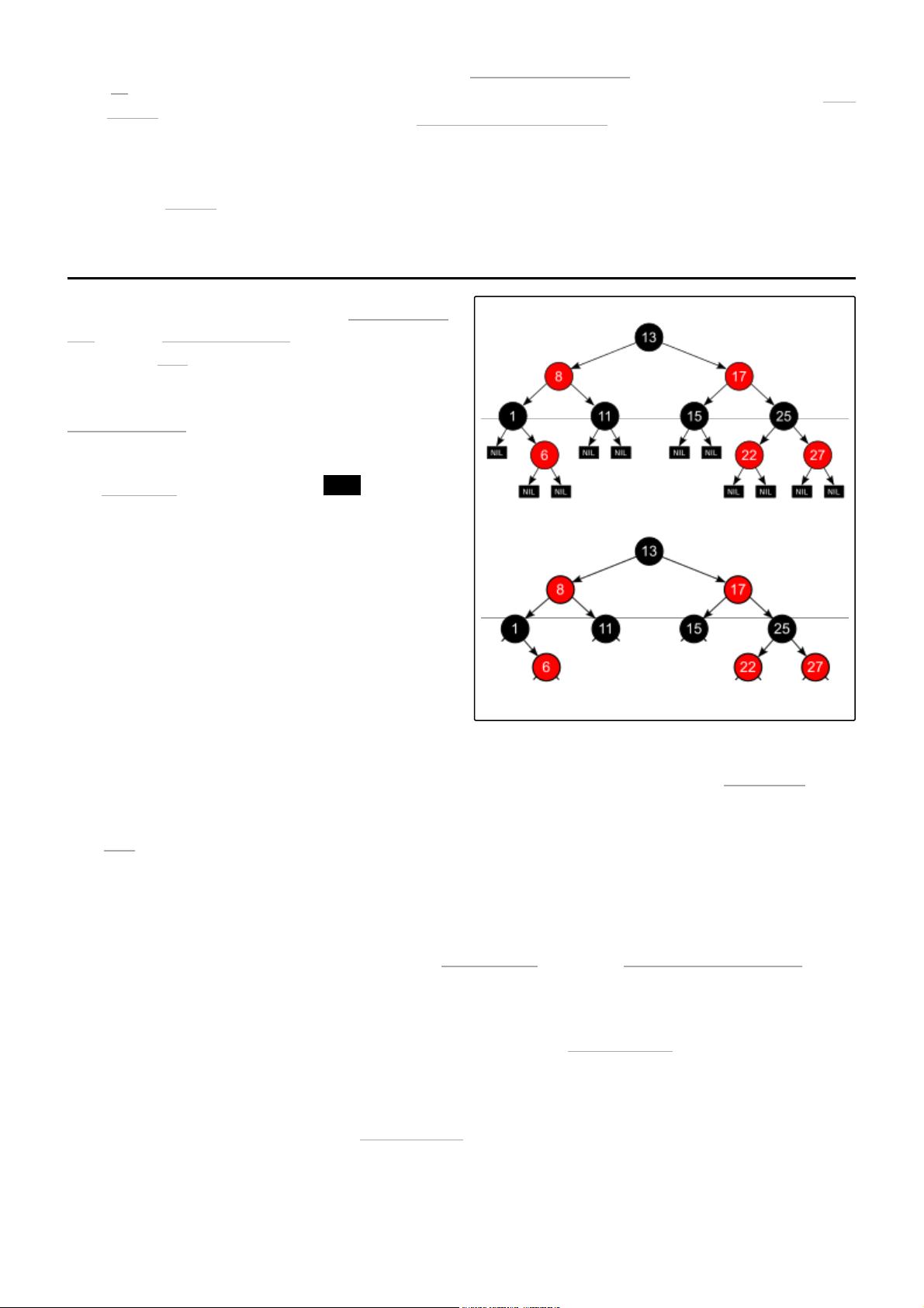
In computer science, a red–black tree is a specialised binary
search tree data structure noted for fast storage and retrieval of
ordered information, and a guarantee that operations will complete
within a known time. Compared to other self-balancing binary
search trees, the nodes in a red-black tree hold an extra bit called
"color" representing "red" and "black" which is used when re-
organising the tree to ensure that it is always approximately
balanced.
[3]
When the tree is modified, the new tree is rearranged and
"repainted" to restore the coloring properties that constrain how
unbalanced the tree can become in the worst case. The properties
are designed such that this rearranging and recoloring can be
performed efficiently.
The (re-)balancing is not perfect, but guarantees searching in Big
O time of , where is the number of entries (or keys) in
the tree. The insert and delete operations, along with the tree
rearrangement and recoloring, are also performed in
time.
[4]
Tracking the color of each node requires only one bit of information per node because there are only two
colors. The tree does not contain any other data specific to it being a red–black tree, so its memory footprint
is almost identical to that of a classic (uncolored) binary search tree. In some cases, the added bit of
information can be stored at no added memory cost.
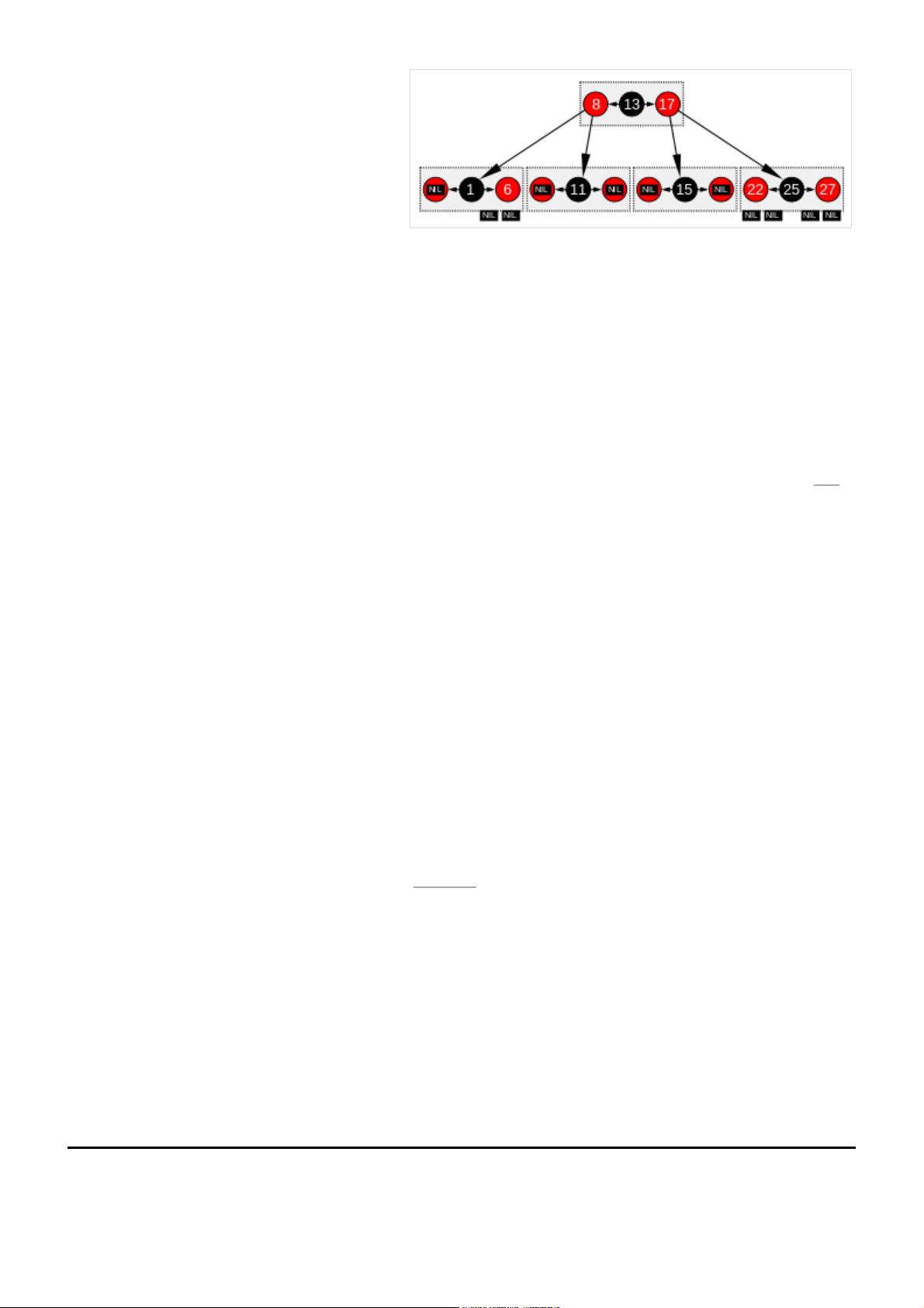
In 1972,
Rudolf Bayer
[5]
invented a data structure that was a special order-4 case of a
B-tree
. These trees
maintained all paths from root to leaf with the same number of nodes, creating perfectly balanced trees.
However, they were not binary search trees. Bayer called them a "symmetric binary B-tree" in his paper
and later they became popular as
2–3–4 trees
or even 2–4 trees.
[6]
In a 1978 paper, "A Dichromatic Framework for Balanced Trees",
[7]
Leonidas J. Guibas
and
Robert
Sedgewick
derived the red–black tree from the symmetric binary B-tree.
[8]
The color "red" was chosen
because it was the best-looking color produced by the color laser printer available to the authors while
working at
Xerox PARC
.
[9]
Another response from Guibas states that it was because of the red and black
pens available to them to draw the trees.
[10]
In 1993, Arne Andersson introduced the idea of a right leaning tree to simplify insert and delete
operations.
[11]
In 1999, Chris Okasaki showed how to make the insert operation purely functional. Its balance function
needed to take care of only 4 unbalanced cases and one default balanced case.
[12]
History
剩余26页未读,继续阅读
资源评论


