没有合适的资源?快使用搜索试试~ 我知道了~
资源推荐
资源详情
资源评论
1
Mechanics
We start with an outline of classical mechanics, to provide a framework for the discrete ele-
ment method (DEM). While most of the material in this chapter can be found scattered in
various books on mechanics, no text seems to be available which covers concisely the con-
cepts needed for DEM simulation. This chapter is intended as a crash course in theoretical
mechanics, with an emphasis on issues relevant to computer implementation and testing. We
give a list of secondary literature that the reader may refer to for further details.
1.1 Degrees of freedom
Before discussing the dynamics of a mechanical system, we need to understand the nature of
the variables in the system. There are independent variables on the one hand, usually called
‘degrees of freedom’, and then there are dependent variables which depend on the degrees of
freedom, via algebraic relations or derivatives.
1.1.1 Particle mechanics and constraints
The concept of a ‘mass point’ means that we neglect the size of the mass and are interested
only in its trajectory. The position of a single mass point moving along the Cartesian x-axis
is described by the value of x, which corresponds to a single degree of freedom. A point
moving in the xy-plane has two degrees of freedom, r
2D
=(x, y), and a point moving in three-
dimensional real space will have three degrees of freedom, r
3D
= (x,y,z).Although we can
describe the motion of a point in three-dimensional space by four ‘space–time coordinates’
using the tuple (x,y,z,t),in classical mechanics t is not considered a degree of freedom but
rather a parameter, i.e. an independent variable which cannot be influenced.
Two mass points moving independently along the x-axis represent two degrees of freedom,
r
1
and r
2
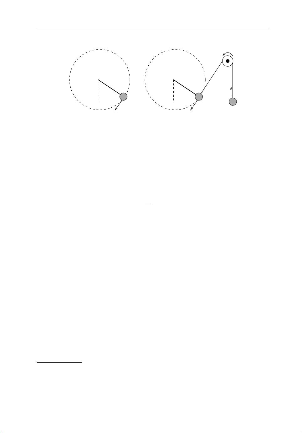
(here and in the following, we assume equal masses). If we ‘glue’ these two particles
together at distance d =r
1
−r
2
as in Figure 1.1, one degree of freedom gets lost, and we are
Understanding the Discrete Element Method: Simulation of Non-Spherical Particles for Granular
and Multi-body Systems, First Edition. Hans-Georg Matuttis and Jian Chen.
© 2014 John Wiley & Sons, Singapore Pte Ltd. Published 2014 by John Wiley & Sons, Singapore Pte Ltd.
Companion website: www.wiley.com/go/matuttis
2 Understanding the Discrete Element Method
n
dof
=2
n
dof
=2∙2–1=3
n
dof
=3·2–3=3
n
dof
=4·2–5=3
Figure 1.1 In two dimensions, the number of degrees of freedom n
dof
for1,2,3or4constrained
particles with an increasing number of constraints introduced. Newly added constraints are in black;
previous constraints are in gray.
left with only a single degree of freedom; in this case we can use either of r
1
, r
2
or the average
(r
1
+r
2
)/2 to determine the position of both particles uniquely. This means that one constraint
between two position variables eliminates one degree of freedom.
In two dimensions, for two point particles at r
1
= (x
1
,y
1
) and r
2
= (x
2
,y
2
) we have four
degrees of freedom, x
1
,y
1
,x
2
and y
2
. If we again fix the distance between the particles at a
constant distance d, so that
(x
2
− x
1
)
2
+ (y
2
− y
1
)
2
= d, (1.1)
we can choose any three variables from {x
1
,y
1
,x
2
,y
2
} and the fourth will then be determined
from (1.1) by elementary geometry. Alternatively, we can introduce new variables, such as
the position of the center of mass, (x, y) = (r
1
+ r
2
)/2 for particles of the same mass, the
displacement (x, y) = (x
2
− x
1
,y
2
− y
1
) between the particles, and the angle θ that the
line segment between the two particles makes with the x-axis. In any case, we end up with
three independent variables to describe the positions of the two particles fully. This means
that a single constraint (1.1) reduces the number of degrees of freedom, i.e. the number of
independent variables in the system, by 1.
In three-dimensional space, for two particles at positions (x
1
,y
1
,z
1
) and (x
2
,y
2
,z
2
) as
shown in Figure 1.2, a constraint
(x
2
− x
1
)
2
+ (y
2
− y
1
)
2
+ (z
2
− z
1
)
2
= d (1.2)
will again reduce the number of degrees of freedom by 1, so if we want to work with the
center of mass
(x,y,z) =
1
2
{
(x
1
,y
1
,z
1
) + (x
2
,y
2
,z
2
)
}
,
we need two angles, φ and θ say, to describe the orientation of the ‘rod’ in space. Rotation
around the orientation of the rod is not a degree of freedom, as it does not change the positions
of the two points. In principle, it does not matter how one defines the degrees of freedom,
whether it is with six variables and one constraint (1.2), with three Cartesian coordinates for
Mechanics 3
n
dof
=3
n
dof
=3∙2–1=5
n
dof
=3·4–6=6
n
dof
=3·3–3=6 n
dof
=3·5–9=6
Figure 1.2 In three dimensions, the number of degrees of freedom n
dof
for 1, 2, 3, 4 or 5 particles
constrained so that the resulting cluster has no internal degrees of freedom. Newly added constraints are
in black; previous constraints are in gray.
the center of mass and two angles, or with three Cartesian coordinates for one endpoint and
two angles. In each case the number of degrees of freedom is the same, namely 5.
1.1.2 From point particles to rigid bodies
When we introduce one more point mass at (x
3
,y
3
,z
3
) to our set-up, we have 9 variables in
total. If we connect this new point to both ends of our rod with the additional constraints
(x
3
− x
1
)
2
+ (y
3
− y
1
)
2
+ (z
3
− z
1
)
2
= d
2
, (1.3)
(x
3
− x
2
)
2
+ (y
3
− y
2
)
2
+ (z
3
− z
2
)
2
= d
3
, (1.4)
we get a triangle, as in the middle diagram of Figure 1.2. Again, we can give an alternative
description of its position in space using the center of mass, and use three angles, φ,θ and ψ,
to describe the orientation. So the formula
(degrees of freedom)
6
= (variables)
9
−(constraints)
3
again holds. If we connect a fourth particle rigidly to the cluster of three particles so that it
does not lie in the plane described by the other three, as shown in the fourth diagram from
the left in Figure 1.2, then the three extra constraints exactly compensate for the additional
three coordinates (x
4
,y
4
,z
4
) of the new particle. In fact, for four or more spatially connected
particles, the total number of degrees of freedom is always 6. Note that the rigid body formed
by the connected particles need not be three-dimensional; for example, although a triangle
is a two-dimensional shape, if it can rotate in three dimensions, then it also has six degrees
of freedom. Through the reasoning above, we have derived that an extended rigid body has
six degrees of freedom, irrespective of its size. The angular degrees of freedom φ,θ,ψ are
obtained from the rectilinear degrees of freedom (x
1
,y
1
,z
1
), (x
2
,y
2
,z
2
), . . . of the particles
upon introducing constraints of finite length between the particles.
4 Understanding the Discrete Element Method
‘Mathematically’ one can define a point particle as an object having ‘zero extension’ and a
rigid body as one having ‘zero deformation’. A more pragmatic definition of a point particle is
an object whose extent is much smaller than the distances that it covers in the processes under
investigation; after all, the Earth is pretty extended, but t he point-mass approach to describing
its trajectory around the sun works rather well. Likewise, a rigid body is an object for which
the deformations are much smaller than the scales that are of interest in the processes being
investigated.
1.1.3 More context and terminology
In principle, a ‘continuum’ has infinitely many degrees of freedom; but in order to solve
continuum problems with a computer, we have to first discretize the continuum to obtain a
finite number of degrees of freedom. We could, for instance, decompose the continuum into
representative mass points and model the elasticity by springs between the mass points. The
deformation of a spring can be computed from the positions of the bodies, so the springs
will not be degrees of freedom, while the coordinates of the mass points will be degrees
of freedom. With a finite element discretization, we decompose the elastic continuum into
a space-filling partition of elements for which elastic stress relations hold, and the degrees
of freedom are the nodes of the elements. Depending on the choice of boundary conditions,
there may be as many nodes as there are elements, or more; therefore, from the nodes one can
calculate the center of mass of the elements, but not vice versa. Describing the physics via the
motion of particles, for example of centers of mass, is called the ‘Lagrangian representation’.
This approach is natural for particulate systems, so we will adopt it in this book. Formulating
the physics for a reference system in which, e.g., density amplitudes change is called the
‘Eulerian representation’; this representation is preferable for many continuum problems. In
a Lagrangian representation, velocities of mechanical bodies are not degrees of freedom: they
can be obtained as the time derivatives of the positions on which they depend. On the other
hand, when we simulate a fluid volume where velocities are assigned to the nodes of a finite
element or finite difference approximation in ‘Eulerian representation’, it is the velocities that
are the degrees of freedom.
In the previous two subsections, we introduced constraints as algebraic relations between
positions, but we remark here that constraints (whose associated functions are usually denoted
by g in formulae) can also be imposed on velocities. For a pendulum of length l swing-
ing around the origin as in Figure 1.3(a), the constraint g(x, y) stating that the bob (whose
diameter we will neglect) stays at constant distance from the origin is
x
2
+ y
2
= l
2
. (1.5)
In § 2.8 we will discuss the numerical solution of a problem where, in addition to constraints
on x and y, constraint relations for ˙x and ˙y are also in effect. In undergraduate mechanics,
it is common to circumvent solving the equations of motion of a constrained system with
variables (x, y) that simultaneously satisfy (1.5) by transforming into plane polar coordinates
(φ, r) so that r is eliminated. For more complicated mechanical systems, such a simplifying
transformation may not be possible any more, for instance if the pendulum is connected with
a unidirectionally moving body as in Figure 1.3(b).
Mechanics 5
l
v
(x, y)
(a)
ϕ
l
v
v
z
(x, y)
(b)
ϕ
z
Figure 1.3 (a) Pendulum as a constrained problem; (b) coupled pendulum–wheel–mass system, where
transformation into polar coordinates does not simplify the calculation.
1.2 Dynamics of rectilinear degrees of freedom
Labeling the coordinates with different letters such as x
1
,y
1
,z
1
,...will soon become incon-
venient, so let us rename them as follows: x
1
= r
(1)
1
,y
1
= r
(2)
1
,z
1
= r
(3)
1
,x
2
= r
(1)
2
,y
2
=
r
(2)
2
,z
2
= r
(3)
2
, ..., where the lower index represents the particle and the upper index in
parentheses represents the dimension. The corresponding velocities can then be obtained as
time derivatives:
v
(j)
i
=
d
dt
r
(j)
i
=˙r
(j)
i
.
If all the velocities vanish, we say that the system is static; if the velocities (which may be
non-zero) do not change, we say that the system is stationary. The accelerations are the time
derivatives of the velocities, or the second derivatives of the positions with respect to time:
a
(j)
i
=˙v
(j)
i
=¨r
(j)
i
. If the acceleration is constant, we also refer to it as ‘uniform’; in this
case the velocity changes at a constant rate. For a particle i with mass m
i
, Newton’s equation
of motion
1
expresses the relationship between the force F
(j)
i
applied to the particle and the
acceleration a
(j)
i
in coordinate j as
F
(j)
i
= m
i
¨x
(j)
i
= m
i
a
(j)
i
.
(1.6)
Numerical analysis prefers to deal with first-order equations, so often it is necessary to rewrite
the second-order equation (1.6) as a first-order system by defining the velocity as an auxiliary
variable:
F
(j)
i
= m
i
˙v
(j)
i
, (1.7)
v
(j)
i
=˙x
(j)
i
. (1.8)
1
This second-order differential equation formulation is actually due to Euler. Newton wrote his second law of motion
as a first-order differential equation F =˙p, where p is the momentum, but mathematically this is not equivalent to
Euler’s formulation.
剩余400页未读,继续阅读
资源评论
- dianxin20232023-06-25资源简直太好了,完美解决了当下遇到的难题,这样的资源很难不支持~
少年小鱼
- 粉丝: 28
- 资源: 532
上传资源 快速赚钱
- 我的内容管理 展开
- 我的资源 快来上传第一个资源
- 我的收益 登录查看自己的收益
- 我的积分 登录查看自己的积分
- 我的C币 登录后查看C币余额
- 我的收藏
- 我的下载
- 下载帮助
安全验证
文档复制为VIP权益,开通VIP直接复制
信息提交成功